Trend tests for raster time series

Applies a trend test to a raster time series – the general step this function exists for, regardless of which specific test is used underneath. trend_test() is the core inferential step of sptrends. In a standard workflow it follows optional preprocessing (compute_anomalies(), prewhiten()) and precedes slope estimation (slope_estimator()) and multiple-testing correction (fdr_correction()).

Usage

trend_test(
  x,
  method = c("CMK", "MK", "OLS", "MMK"),
  ties = FALSE,
  t = NULL,
  window_size = 3L,
  connectivity = c("queen", "rook"),
  precomputed_neighbourhood = NULL,
  continuity = FALSE,
  n_cores = 1,
  alpha = c(0.1, 0.05, 0.01),
  report = TRUE,
  verbose = TRUE,
  shared_cluster = NULL
)

Arguments

x

A terra::SpatRaster; each layer is one time step, in increasing chronological order.

method

Which trend test to run. "CMK" is the default for spatially coherent gridded data; "MK", "OLS", and "MMK" address the distinct cases described below and are not equally weighted substitutes.

"CMK" (default): full Contextual Mann-Kendall using a square queen neighbourhood. window_size = 3L reproduces the region described by Neeti and Eastman (2011), as implemented in TerrSet's Kendall module, with at most m = 9: the focal cell plus eight valid neighbours. Larger odd windows extend the same CMK equations to a broader region, as explicitly anticipated by Neeti and Eastman (2011). "MK": classic cell-by-cell Mann-Kendall (no spatial averaging) – the foundational statistic "CMK" builds on. "OLS": the classical parametric alternative – a per-cell ordinary least squares regression against t, with the standard t-test on the slope coefficient (n - 2 degrees of freedom); like "MK", no spatial averaging. "MMK": the modified Mann-Kendall test of Hamed and Rao (1998) – corrects the classical MK test's own variance formula for temporal autocorrelation directly (an effective sample size, estimated from the significant autocorrelation of the Sen-detrended series' own ranks), rather than transforming the series the way prewhiten() does; like "MK", no spatial averaging.

"MMK" is an alternative to prewhitening, not a complement to it: do not run prewhiten() before using method = "MMK". Both exist to solve the same problem – temporal autocorrelation inflating the classical MK test's significance – by different means; "MMK" corrects the test statistic's own variance directly, without transforming the data first. Running it on an already-prewhitened series applies that correction to data with little autocorrelation left to detect (at best redundant), or compounds two corrections for the same issue (at worst biased) – see "Methodological details" below.

Use "CMK" when neighbouring cells are expected to exhibit coherent trends (the usual case for environmental rasters, and this function's own recommendation for that case – see "Methodological details" below). Use "MK" when reproducing the classic Mann-Kendall test, or when spatial pooling is not appropriate for the data at hand (e.g. cells that are not genuinely spatially related to one another). Use "OLS" when the residuals are genuinely expected to be close to normally distributed with no substantial outlier risk (in which case OLS is the more statistically efficient of the three), or when the result needs to be directly comparable to other analyses reported as classical linear-regression trend tests – see slope_estimator()'s own method argument for the same robust-vs-parametric trade-off applied to slope estimation instead of significance testing. Use "MMK" as an alternative to prewhitening when temporal autocorrelation is suspected but a spatial-pooling assumption ("CMK"'s own) is not appropriate, or when comparing against published studies reporting this particular correction.

ties

Logical. Only used when method is "CMK", "MK" or "MMK". FALSE (default): closed-form variance (Eq. 3). TRUE: correct for tied (repeated) values within each cell's time series (Eq. 4) – relevant for low numeric-resolution variables. For CMK, every cell's resulting VarS is propagated through the complete RAMK covariance sum, so neighbouring series may have different tie-corrected variances. This option is slower because tie groups are calculated row by row. Most continuous environmental variables (NDVI, temperature, precipitation) rarely need this correction, since exact ties are uncommon at typical measurement precision.

t

Numeric vector of time points, one per layer. Only used when method is "OLS" or "MMK" ("CMK"/"MK" are rank-based and need only the chronological order of layers, not their actual spacing; "MMK" needs t for its own Sen-slope detrending step, even though its significance test that follows is, like "MK", rank-based). Defaults to 1:nlyr(x) (evenly-spaced steps) if NULL. Supply real time values here if layers are not evenly spaced (e.g. a gap for a missing year) – unlike "CMK"/"MK", OLS's own slope and its significance depend on the actual spacing, not just the order. Values must be finite, unique and strictly increasing.

window_size

Odd integer greater than or equal to 3. Width and height, in raster cells, of the square neighbourhood used only by method = "CMK" (see connectivity below for its shape). The default 3L preserves the CMK region described by Neeti and Eastman (2011), as implemented in TerrSet's Kendall module. Larger values such as 5L or 7L change the spatial scale of the contextual test; choose them from the process scale and raster resolution, not as automatic upgrades. A non-default value with another method is rejected.

connectivity

"queen" (default, 8 neighbours) or "rook" (4 neighbours, no diagonals). Only used when method = "CMK". "queen" preserves the CMK region described by Neeti and Eastman (2011); "rook" is a narrower neighbourhood, useful when diagonal-only adjacency is not a meaningful spatial relationship for the process being tested, or to check how sensitive a result is to the choice of neighbourhood shape. A non-default value with another method is rejected.

precomputed_neighbourhood

Optional output of prepare_cmk_neighbourhood(), to avoid recomputing the adjacency when this function is called repeatedly on the same raster (e.g. in a permutation loop). It does not alter the statistical method in any way; it only skips rebuilding the spatial adjacency structure that method = "CMK" needs. Only used when method = "CMK". If NULL (typical single-call use), it is computed internally. Reuse is accepted only when matrix dimensions, raster geometry, the requested connectivity, window_size, and the complete-case cell pattern all match x; incompatible objects produce an error rather than a result built from the wrong neighbours.

continuity

Logical. Only used when method = "CMK". Default FALSE: Zm is computed as Sm / sqrt(VarSm), Eq. 10 exactly as published (Neeti and Eastman, 2011) – see "Implementation notes" below for why the continuity correction reserved for the single-cell classic MK statistic (Eq. 5) is not applied to the neighbourhood-averaged Sm. Set to TRUE to apply it anyway (Zm = (Sm +- 1) / sqrt(VarSm)), matching ConMK's own convention instead – see "External validation" below, including inst/validation/ for a reproducible, cell-by-cell comparison confirming the match for neighbourhoods without zero-variance series. At Sm = 0, this option deliberately follows ConMK's +1 branch rather than forcing Z = 0. This is an opt-in for matching another implementation's convention, not a recommendation to prefer it over this function's own default.

n_cores

Integer. Number of cores to use for the S-statistic computation (the O(n^2) loop over pairs of time steps). Only used when method is "CMK", "MK" or "MMK" – "OLS"'s own per-cell fit is already a single vectorised matrix operation across every cell at once, with no comparable loop to parallelise. 1 (default): sequential, identical to the original implementation. > 1: splits the outer loop across a parallel::makeCluster() PSOCK cluster (works on Windows, macOS, and Linux). Only worth it for long time series (large n) and/or very large rasters, since each worker needs a copy of the full data matrix.

alpha

Numeric vector of significance thresholds. What it controls: only used when report = TRUE, passed to trend_summary() as-is. How it is used for maps: the single threshold for trend_maps() is 0.05 if it is one of the values in alpha (the default vector includes it), otherwise the strictest (smallest) value supplied. The default c(0.1, 0.05, 0.01) reports all three side by side for context, but they are not interchangeable defaults – 0.05 is the conventional standard and the one used for the map; 0.1 is a more liberal threshold not unusual in exploratory trend studies (more power to detect a trend, at the cost of more false positives); 0.01 is markedly more conservative. Why not a final result: every value here is uncorrected for multiple testing – see "Methodological details" above; do not treat cells crossing alpha here as a final significance map.

report

Logical. If TRUE (default), automatically print the summary table (trend_summary()) and draw the diagnostic histograms and maps (trend_histograms(), trend_maps()) after computing. Set to FALSE for programmatic use (e.g. inside a loop, or when called from workflow_tst()).

verbose

Logical. Print progress messages and elapsed time.

shared_cluster

Advanced; most users never need this directly. An already-running parallel::makeCluster() PSOCK cluster (e.g. from workflow_tst()'s own n_cores) to reuse instead of building a new one from n_cores above. When supplied, n_cores is ignored – the shared cluster's own size was already decided by whoever built it. NULL (default): builds and tears down its own cluster from n_cores, exactly as before this argument existed.

Value

Returns a list of class c("trend_test", "sptrends"), with:

stats: A 3-layer SpatRaster: Sm, VarSm, p for method = "CMK"; S, VarS, p for method = "MK" or "MMK" (VarS is the Hamed-and-Rao-corrected variance for "MMK", the uncorrected closed-form variance for "MK"); beta (the OLS slope estimate), se_beta (its standard error), p for method = "OLS".
neighbourhood: Logical: TRUE if method = "CMK" (spatial averaging was used), FALSE for "MK", "MMK" and "OLS".
window_size: The odd CMK neighbourhood size used, or NULL for non-CMK methods.
method: The requested trend-test method.
connectivity: For CMK, the selected queen or rook connectivity.

Use print()/summary()/plot() – see print.sptrends(), summary.sptrends(), and plot.sptrends() – rather than accessing $stats directly for anything beyond programmatic use.

Details

Four tests are available through one interface: Contextual Mann-Kendall ("CMK", the default), classic Mann-Kendall ("MK"), ordinary least squares ("OLS"), and modified Mann-Kendall ("MMK"). They answer the same broad question – whether change over time is statistically distinguishable from no trend – but make different assumptions. See method and "Methods and method selection" below.

Function type: Core function – one of the core building blocks of TST and RTA. Typically followed by fdr_correction(), once this function's own p-values exist for every spatial cell.

Typical use

raster time series
    |
trend_test()
    |
test statistics + raw p-value raster (`result$stats$p`)
    |
fdr_correction()

Use prewhiten() first when serial correlation requires treatment, except when choosing method = "MMK", which is itself the alternative variance correction; analyse the prewhitened result$series with the other methods. Estimate change magnitude separately with slope_estimator(); significance and slope answer different questions.

Methodological details

What CMK tests

CMK tests the null hypothesis of no monotonic trend for every focal raster cell while using the focal cell's local spatial context. It does not smooth or replace the observed values. Instead, it combines the Mann-Kendall evidence from the focal cell and its immediate neighbours, then adjusts the variance for correlation among those series. A positive pooled statistic (Sm) indicates a predominantly increasing local region; a negative value indicates a predominantly decreasing one. The returned p tests whether that local regional statistic is compatible with no monotonic trend.

The geographical rationale is that many environmental processes are spatially continuous: if a trend is real, nearby cells will often contain related evidence. CMK can therefore gain power over isolated cell-wise MK when this assumption is justified. It must not be used merely because the input is a raster: boundaries, fragmented habitats, categorical mosaics, or other abrupt spatial discontinuities can make neighbouring trends legitimately different. Use "MK" in those cases.

CMK and prewhitening – two separate operations

trend_test(method = "CMK") does not prewhiten the series. This point is easy to misunderstand from Neeti and Eastman (2011). Their article presents prewhitening and contextual significance testing together in one broader analytical procedure: the discussion and flowchart first address serial autocorrelation and then apply CMK to the resulting series. That presentation can make prewhitening look like an internal part of CMK. It is not. The defining CMK equations (their Eqs. 7-13) contain the local average of Kendall statistics, the cross-correlation-adjusted variance, and its standardisation; they contain no prewhitening transformation.

The two operations address different dependencies:

serial autocorrelation is dependence through time within one cell; diagnose and, when justified, treat it before this function with prewhiten(), or use "MMK" as a non-prewhitening alternative;
spatial cross-correlation is contemporaneous dependence between different cells; CMK accounts for it in VarSm.

Prewhitening one cell at a time does not remove the lag-zero cross-correlation between neighbouring cells. Conversely, CMK's spatial variance adjustment does not remove serial autocorrelation. A workflow that needs both therefore calls prewhiten() first and trend_test(method = "CMK") second. Keeping them as separate, composable functions makes the statistical role of each step explicit.

Relationship between CMK and RAMK

CMK is the moving-window raster application of the analytical Regionally Averaged Mann-Kendall (RAMK) test of Douglas, Vogel and Kroll (2000). The mathematical logic is shared:

calculate Kendall's S for every series in a region;
average those statistics to obtain the regional statistic;
include all within-region cross-covariances in its variance;
standardise the regional statistic and obtain a p-value.

RAMK applies this calculation once to a predefined group of stations. CMK moves the region across a raster and returns one result per focal cell. With the default complete 3 by 3 queen neighbourhood, the local region contains nine series: the focal cell plus eight neighbours. Larger odd window_size values use the corresponding square region. At raster edges or beside missing cells, m is the number actually available, so incomplete regions are not silently treated as complete. This function is therefore an analytical RAMK calculation for each local raster region under the common-length conditions and covariance formulation developed in both papers; it is not a general RAMK interface for arbitrary station regions.

How CMK is calculated

For each valid cell, trend_test() performs the following steps.

Compute the ordinary Mann-Kendall statistic S from all ordered pairs of time steps. No slope magnitude enters this statistic.
Define the local square region from the focal cell and the valid queen neighbours within window_size.
Compute Sm as the mean of the S statistics in that region (Neeti and Eastman Eq. 7; Douglas et al. Eq. 7).
Estimate every lag-zero cross-correlation among the regional series and include the corresponding covariance terms in VarSm (Neeti and Eastman Eqs. 11-13; Douglas et al. Eqs. 11-13). When ties are corrected, each pair uses rho[i,j] * sqrt(VarS[i] * VarS[j]); thus different tie patterns may give different cell-wise variances without imposing the focal cell's variance on the rest of the region.
By default, calculate Zm = Sm / sqrt(VarSm) and its two-sided normal-approximation p-value.

The covariance adjustment is essential. Treating neighbouring series as independent would underestimate the uncertainty of their pooled statistic and create too many apparently significant trends. The correction is analytical and relies on the assumptions stated in the source methods; it should be interpreted as a model-based variance adjustment, not as proof that all forms of spatial dependence have disappeared.

Statistical assumptions and interpretation

for every method, layers are ordered chronologically, represent comparable time steps, and valid cells have complete series;
for "CMK", "MK", and "MMK", the trend of interest is monotonic, not necessarily linear, and the normal approximation is adequate for the available record;
for "CMK", local spatial coherence is scientifically defensible;
for "CMK" and "MK", serial autocorrelation has been assessed separately; "MMK" instead adjusts the rank-test variance for it;
for "OLS", the temporal relationship is linear and the usual regression-inference assumptions concerning residual independence, constant variance, and approximate normality are defensible;
raw cell-wise p-values are followed by a multiple-testing procedure such as fdr_correction() before producing a final significance map.

Sm describes direction and strength on the Mann-Kendall rank scale, not change per year. Use slope_estimator() for magnitude. A small p supports a locally coherent monotonic trend; it does not establish causation, practical importance, linearity, or a particular slope.

This is an independent implementation of the published equations. It is not affiliated with the original authors and does not port code from TerrSet's Kendall module.

Methods and method selection

Original publication: Neeti & Eastman (2011), the "Contextual Mann-Kendall" (CMK) extension of the classic Mann-Kendall test.
Why "CMK" is this function's own default and recommendation: gridded environmental data (the case this package is built around) routinely shows spatial autocorrelation – a real trend at one cell is expected, not merely permitted, to look similar to its immediate neighbours (Tobler's first law). CMK is designed to use that expected structure to its advantage, borrowing statistical strength across the neighbourhood while adjusting the test statistic's own variance to keep the significance decision formally valid – see "Methodological details" above for the mechanism. "MK" is the right choice specifically when that spatial expectation does not hold for the data at hand (see "Why method = \"mk\" remains available" below), not as an equally-good default.
Why method = "MK" remains available: classic Mann-Kendall is the reference method in the literature, with the longest track record and the simplest assumptions (no spatial pooling at all). "CMK" is not a strict replacement for it – see the method argument below for when each is the more defensible choice.
Why method = "OLS" is offered too: "CMK"/"MK" are both rank-based (built on the Mann-Kendall S statistic), robust to outliers and non-normal noise – this package's own default assumption about gridded environmental data, and the reason "CMK"/"MK" are recommended ahead of "OLS" in general. "OLS" is the classical parametric alternative – the standard significance test for a linear regression slope – offered for the specific, narrower case where that robustness genuinely is not needed (see the method argument below), the same reason slope_estimator() offers Theil-Sen, OLS, and Siegel's repeated median rather than only one robust option: this package aims to be a platform for comparing such methods (see compare_detections()), not a vehicle for only one statistical philosophy.
Why method = "MMK" is offered, and why it is an alternative to prewhitening, not a complement: temporal (not spatial) autocorrelation is a separate problem from the one CMK addresses, and this package's other answer to it is prewhiten() – which transforms the series before testing it. "MMK" (Hamed and Rao, 1998) solves the same problem differently: it leaves the series untouched and corrects the classical MK test's own variance formula directly, using an effective sample size derived from the autocorrelation remaining in a Sen-detrended version of the ranks. Because both correct for the same underlying issue by different mechanisms, applying both together (prewhitening the series and then also using "MMK") is not additive – see the method argument below for when "MMK" is the more appropriate choice on its own.
Main references: Douglas, Vogel & Kroll (2000) for the Regionally Averaged Mann-Kendall (RAMK) statistic and its cross-correlation-adjusted variance; Neeti & Eastman (2011) for applying that analytical RAMK logic as CMK in a moving 3 by 3 raster neighbourhood, while explicitly noting that the technique can be extended to any neighbourhood size (CMK itself does not prewhiten); Mann (1945) and Kendall (1975) for the foundational statistic "CMK"/ "MK" extend; Tobler (1970) for the spatial-coherence rationale behind averaging with the neighbourhood; Legendre (1805) and Gauss (1809) for the classical least-squares regression "OLS" is built on; Hamed and Rao (1998) for "MMK". Full citations appear under "References" below.
Typical applications: trend detection in gridded remote sensing and climate time series, where a genuine trend is expected to be spatially coherent rather than isolated in a single pixel.

Monotonic trends only – deseasonalise first if needed

Mann-Kendall (and its contextual variant here) tests for a monotonic trend: a consistent tendency to increase or to decrease over time. It is not designed to detect or accommodate a periodic/seasonal cycle – if the input has one (e.g. raw monthly data with an annual cycle), that cycle itself will dominate the ranking of values and can produce a meaningless or misleading trend result. Deseasonalise first (see compute_anomalies()) and run this function on the anomalies, not on the raw seasonal series.

Implementation notes

Eq. 10 (Zm = Sm / sigma_m) is implemented as written, without the continuity correction: confirmed directly against Neeti and Eastman's own text for Eqs. 7-10, which introduce Sm, its mean and variance, and Zm with no +-1 term anywhere in that derivation – the continuity correction belongs to the single-cell classic MK statistic (Eq. 5) specifically, whose discrete step-2 structure motivates it; Sm, being an average across a neighbourhood, loses that structure. Cells with a constant time series (zero variance) would otherwise produce NaN correlations that propagate to their valid neighbours; here the zero standard deviation is replaced by Inf before dividing, giving a well-defined zero correlation. The neighbour-neighbour covariance term is computed via a closed-form identity that avoids an O(k^2) loop per cell, and the whole variance adjustment uses sparse matrix multiplication (package Matrix) rather than a tapply() loop.

External validation

ConMK (Antiphon, GitHub, https://github.com/antiphon/ConMK, not on CRAN): the strongest external check available for this function, since its C++ source was inspected directly rather than trusted from its own documentation. S/Sm matched to floating-point precision on 100 cells of simulated data. The bundled frozen comparison records S/Sm and p; the accompanying script also records both variance estimates when the comparison is re-run. p differed for 97 of the 100 cells (the remaining 3 have Sm near zero, where the correction below crosses zero and produces the opposite-signed effect instead), traced to a specific line in ConMK's own source (Z = (Sm +- 1) / sqrt(s2), a continuity correction this function deliberately omits – see "Implementation notes" above, confirmed directly against Eqs. 7-10). Not a bug in either implementation: ConMK applies the correction meant for the single-cell classic MK statistic to the neighbourhood-averaged one instead, a different choice from what Eq. 10 itself specifies. Set continuity = TRUE (see that argument above) to reproduce ConMK's continuity convention. An automated regression test matches its frozen p values for the 91 cells whose neighbourhoods contain no constant series. One narrow, documented exception: for the 9 of 100 cells in that comparison affected by a constant (zero-variance) neighbouring cell, the cross-correlation term either implementation needs is undefined (0/0); this package's own convention (zero standard deviation replaced with Inf, giving zero correlation – see "Implementation notes" above) is not asserted to match ConMK's own, unknown, handling of the same undefined case.

TerrSet's own Kendall module (Eastman's own reference implementation): method = "MK" (no spatial pooling) matched TerrSet's own classic Kendall module exactly on the same 100 cells, including p. The contextual case (method = "CMK", TerrSet's own KENDALL_Crosscorrelation module) did not match as cleanly, and with no consistent, explainable pattern the way the ConMK difference has – but TerrSet is closed-source, and its own intermediate values (the pooled statistic and its own variance, analogous to this function's Sm/VarSm) are not exposed for inspection, only the final Z/p. Becoming free to use in 2024 (as "liberaGIS") did not make its own source available – what is published on GitHub is the installer and user guide, not the analytical modules' own code. Without the intermediate values, this difference cannot be traced to a specific formula choice the way the ConMK one was, and is reported here as an unresolved, inconclusive observation, not a confirmed discrepancy – closed, unverifiable code is not treated as a ground truth this function's own output is expected to match.

Independent re-confirmation (2026): a separate, freshly-run comparison against an installed copy of ConMK – not a reuse of the frozen comparison above – reproduced both findings on new simulated data. On a 10x10 grid (no continuity correction): S matched to floating-point precision (correlation 1, maximum absolute difference 0) across every cell; p correlated at 0.998, with a maximum absolute difference of 0.087 in the general case (consistent with the continuity-correction difference already documented above, not a new discrepancy). On a separate 15x15 null field with continuity = TRUE: of the cells landing exactly on Sm == 0, ConMK's own p matched this package's p to seven decimal places at every one of them, directly confirming (not just tracing to source code, as before) that continuity = TRUE reproduces ConMK's own convention exactly at this specific edge case, not only in the aggregate.

Computational considerations

A complete window_size by window_size region contains up to window_size^2 series including the focal cell. Increasing the window therefore enlarges the sparse adjacency and every regional covariance calculation; runtime and memory do not remain constant. Start with the default 3 by 3 region and benchmark broader scales on representative data.

Observed execution time versus TerrSet: in the like-for-like validation run, using the same input raster, this implementation of CMK completed substantially faster than TerrSet's contextual Kendall module. This is a practically important advantage for large raster series. It is reported as an observed comparison rather than a universal benchmark: absolute speed and the ratio between programs depend on hardware, raster dimensions, storage, software versions, and the parallel settings used.

Quality assurance

The implementation is exercised at several independent levels:

hand-calculated tests verify S, tie-corrected VarS, Sm, VarSm, and their p-values;
an equation-level test verifies that the centre cell of a 3 by 3 CMK window equals a direct analytical RAMK calculation for the same region;
regression tests verify that the default and explicit 3 by 3 results are identical, and that 5 by 5 regions use the expected valid cells;
classic MK is compared with Kendall::MannKendall() and trend::mk.test();
CMK is compared cell by cell with the open-source ConMK implementation, with its continuity convention tested separately;
rkt independently verifies the regional score aggregation (S / m = Sm); its Hirsch-Slack corrected variance is deliberately not required to equal CMK's analytical RAMK variance;
the classic TerrSet Kendall result is recorded as an exact external match; this is only a partial TerrSet validation because its closed-source contextual result, which exposes neither Sm nor VarSm, is retained as an inconclusive comparison;
automated tests cover ties, constant series, missing and isolated cells, raster edges, queen and rook adjacency objects, serial versus parallel execution, continuity choices, reporting, and returned object structure.

Frozen external results and their reproducible script are stored in inst/validation/. Package-wide checks also include the complete testthat suite, coverage inspection, R CMD check, goodpractice, lintr, and spelling review; see ?sptrends for the overall quality policy. A tool being part of that policy does not imply that a particular source archive has passed its latest run: release-specific results are recorded only after an actual run in cran-comments.md.

Limitations and scope

It does not prewhiten the series for serial correlation (see prewhiten()), does not correct for multiple testing (see fdr_correction()), and does not compute a separate robust estimate of trend magnitude such as the Theil-Sen slope. The "OLS" branch necessarily returns its fitted slope (beta), but robust and method-independent magnitude estimation belongs to slope_estimator().

CMK defaults to the local queen 3 by 3 region described in the source paper, as implemented in TerrSet's Kendall module. Neeti and Eastman (2011) explicitly state that the technique can be extended to any neighbourhood size, so larger odd window_size values apply the same equations at a broader spatial scale. This changes the scale of inference: larger windows can stabilise broad regional signals but may dilute small or spatially heterogeneous trends. At edges and beside invalid cells the available region becomes smaller. "MK", "MMK", and "OLS" do not perform spatial pooling. None of the four methods, by itself, controls multiplicity across the returned raster.

Multiple testing: the p-values and alpha thresholds are uncorrected

This applies identically to all four methods ("CMK", "MK", "OLS", and "MMK") – the problem below is about how many tests were run, not about which test statistic each one used.

What alpha is: the significance threshold (e.g. 0.05) is the pre-specified Type I error rate of a test under a true null hypothesis. It is not the posterior probability that a detected trend is false, and its single-test guarantee does not automatically extend to a raster-wide family of tests.

The error that follows from using it directly here: this function returns one test for every valid cell – a raster with thousands of cells means thousands of simultaneous tests, not one. CMK results are also spatially related through overlapping local regions; "cell-wise" does not mean statistically independent. Reading alpha against p cell by cell, with no adjustment for that total count, is a form of selective inference: some cells will cross any fixed alpha purely by chance, regardless of whether a real trend is present anywhere, and deciding significance cell by cell without accounting for how many tests were run leaves both the family-wise error rate and the false discovery rate uncontrolled. Consequently, an unknown fraction of the cells called "significant" this way may be false discoveries. The summary and maps produced when report = TRUE describe this uncorrected result only, not a defensible final significance map, whichever method was used to produce them.

What to do about it: always run fdr_correction() on p before reporting which cells are "significant" – see Gutiérrez-Hernández & García (2025) below for the full statistical argument (this exact problem, in this exact context, is what that paper is about).

References

Foundational statistic this method builds on (the S/VarS this function computes, before the neighbourhood adjustment below):

Mann, H.B. (1945) Nonparametric tests against trend. Econometrica, 13(3), 245-259. doi:10.2307/1907187
Kendall, M.G. (1975) Rank Correlation Methods (4th edn). Charles Griffin, London. No DOI available (pre-DOI-era publication).

Primary method reference:

Neeti, N. and Eastman, J.R. (2011) A Contextual Mann-Kendall Approach for the Assessment of Trend Significance in Image Time Series. Transactions in GIS, 15(5), 599-611. doi:10.1111/j.1467-9671.2011.01280.x

method = "OLS": the classical least-squares regression this test's own t-test is built on, independently attributed to both of the following (no single original paper; both pre-DOI-era):

Legendre, A.M. (1805) Nouvelles méthodes pour la détermination des orbites des comètes. Firmin Didot, Paris.
Gauss, C.F. (1809) Theoria motus corporum coelestium in sectionibus conicis solem ambientium. Perthes und Besser, Hamburg.

method = "MMK":

Hamed, K.H. and Rao, A.R. (1998) A modified Mann-Kendall trend test for autocorrelated data. Journal of Hydrology, 204(1-4), 182-196. doi:10.1016/S0022-1694(97)00125-X

Conceptual grounding for the spatial-coherence rationale behind averaging with the neighbourhood:

Tobler, W. (1970) A Computer Movie Simulating Urban Growth in the Detroit Region. Economic Geography, 46(sup1), 234-240. doi:10.2307/143141

Source of the Regionally Averaged Mann-Kendall (RAMK) regional statistic and its analytical cross-correlation variance correction; CMK applies the same equations to a moving local raster region:

Douglas, E.M., Vogel, R.M. and Kroll, C.N. (2000) Trends in Floods and Low Flows in the United States: Impact of Spatial Correlation. Journal of Hydrology, 240(1-2), 90-105. doi:10.1016/S0022-1694(00)00336-X

Official software implementation (this function is an independent re-implementation of the published equations, not a port of this module's code):

Eastman, J.R. (2016) TerrSet Geospatial Monitoring and Modeling System: Kendall module. Clark Labs, Clark University, Worcester, MA.

On why the uncorrected alpha/p from this function should not be read as a final significance result (see "Methodological details" above):

Gutiérrez-Hernández, O. and García, L.V. (2025) The ghost of selective inference in spatiotemporal trend analysis. Science of The Total Environment, 958, 177832. doi:10.1016/j.scitotenv.2024.177832

This function is used (not authored) by the following studies, which can serve as applied examples of the Contextual Mann-Kendall test in practice:

Gutiérrez-Hernández, O. and García, L.V. (2025) Uncovering true significant trends in global greening. Remote Sensing Applications: Society and Environment, 37, 101377. doi:10.1016/j.rsase.2024.101377
Gutiérrez-Hernández, O., & García, L.V. (2024) Robust Trend Analysis in Environmental Remote Sensing: A Case Study of Cork Oak Forest Decline. Remote Sensing, 16(20), 3886. doi:10.3390/rs16203886
Gutiérrez-Hernández, O. and García, L.V. (2025, September 17) Multiple Testing in Remote Sensing: Addressing the Elephant in the Room. Available at SSRN: https://ssrn.com/abstract=4891512. doi:10.2139/ssrn.4891512
Gutiérrez-Hernández, O., & García, L.V. (2025) False discovery rate estimation and control in remote sensing: reliable statistical significance in spatially dependent gridded data. Remote Sensing Letters, 16(5), 537-548. doi:10.1080/2150704X.2025.2478664
Gutiérrez-Hernández, O., & García, L.V. (2025) Implementing the Linear Adaptive False Discovery Rate Procedure for Spatiotemporal Trend Testing. Mathematics, 13(22), 3630. doi:10.3390/math13223630
Gutiérrez-Hernández, O., & García, L.V. (2026) Intensified and Extended Growing Seasons in Abies marocana Forests (2000-2024): A Robust Seasonal Trend Analysis Using 16-Day MODIS EVI Time Series. Remote Sensing, 18(12), 2052. doi:10.3390/rs18122052

Examples

# \donttest{
# Annual mean NDVI from the bundled environmental dataset.
r <- read_ordered_stack(example_data("vhp_ndvi"))
#> Temporal order auto-detected with pattern '(19[0-9]{2}|20[0-9]{2})'.
#> Automatic mode: order detected from file names. For higher reliability -- especially if the series is not annual -- supplying 'files' explicitly (with 'time' or 'cycle_type') is recommended. See ?read_ordered_stack.
#> Temporal order verification (mandatory, cannot be skipped):
#>  stack_position detected_number                         file
#>               1            1982 VHP_SMN_annual_ndvi_1982.tif
#>               2            1983 VHP_SMN_annual_ndvi_1983.tif
#>               3            1984 VHP_SMN_annual_ndvi_1984.tif
#>               4            1985 VHP_SMN_annual_ndvi_1985.tif
#>               5            1986 VHP_SMN_annual_ndvi_1986.tif
#>               6            1987 VHP_SMN_annual_ndvi_1987.tif
#>               7            1988 VHP_SMN_annual_ndvi_1988.tif
#>               8            1989 VHP_SMN_annual_ndvi_1989.tif
#>               9            1990 VHP_SMN_annual_ndvi_1990.tif
#>              10            1991 VHP_SMN_annual_ndvi_1991.tif
#>              11            1992 VHP_SMN_annual_ndvi_1992.tif
#>              12            1993 VHP_SMN_annual_ndvi_1993.tif
#>              13            1994 VHP_SMN_annual_ndvi_1994.tif
#>              14            1995 VHP_SMN_annual_ndvi_1995.tif
#>              15            1996 VHP_SMN_annual_ndvi_1996.tif
#>              16            1997 VHP_SMN_annual_ndvi_1997.tif
#>              17            1998 VHP_SMN_annual_ndvi_1998.tif
#>              18            1999 VHP_SMN_annual_ndvi_1999.tif
#>              19            2000 VHP_SMN_annual_ndvi_2000.tif
#>              20            2001 VHP_SMN_annual_ndvi_2001.tif
#>              21            2002 VHP_SMN_annual_ndvi_2002.tif
#>              22            2003 VHP_SMN_annual_ndvi_2003.tif
#>              23            2004 VHP_SMN_annual_ndvi_2004.tif
#>              24            2005 VHP_SMN_annual_ndvi_2005.tif
#>              25            2006 VHP_SMN_annual_ndvi_2006.tif
#>              26            2007 VHP_SMN_annual_ndvi_2007.tif
#>              27            2008 VHP_SMN_annual_ndvi_2008.tif
#>              28            2009 VHP_SMN_annual_ndvi_2009.tif
#>              29            2010 VHP_SMN_annual_ndvi_2010.tif
#>              30            2011 VHP_SMN_annual_ndvi_2011.tif
#>              31            2012 VHP_SMN_annual_ndvi_2012.tif
#>              32            2013 VHP_SMN_annual_ndvi_2013.tif
#>              33            2014 VHP_SMN_annual_ndvi_2014.tif
#>              34            2015 VHP_SMN_annual_ndvi_2015.tif
#>              35            2016 VHP_SMN_annual_ndvi_2016.tif
#>              36            2017 VHP_SMN_annual_ndvi_2017.tif
#>              37            2018 VHP_SMN_annual_ndvi_2018.tif
#>              38            2019 VHP_SMN_annual_ndvi_2019.tif
#>              39            2020 VHP_SMN_annual_ndvi_2020.tif
#>              40            2021 VHP_SMN_annual_ndvi_2021.tif
#>              41            2022 VHP_SMN_annual_ndvi_2022.tif
#>              42            2023 VHP_SMN_annual_ndvi_2023.tif

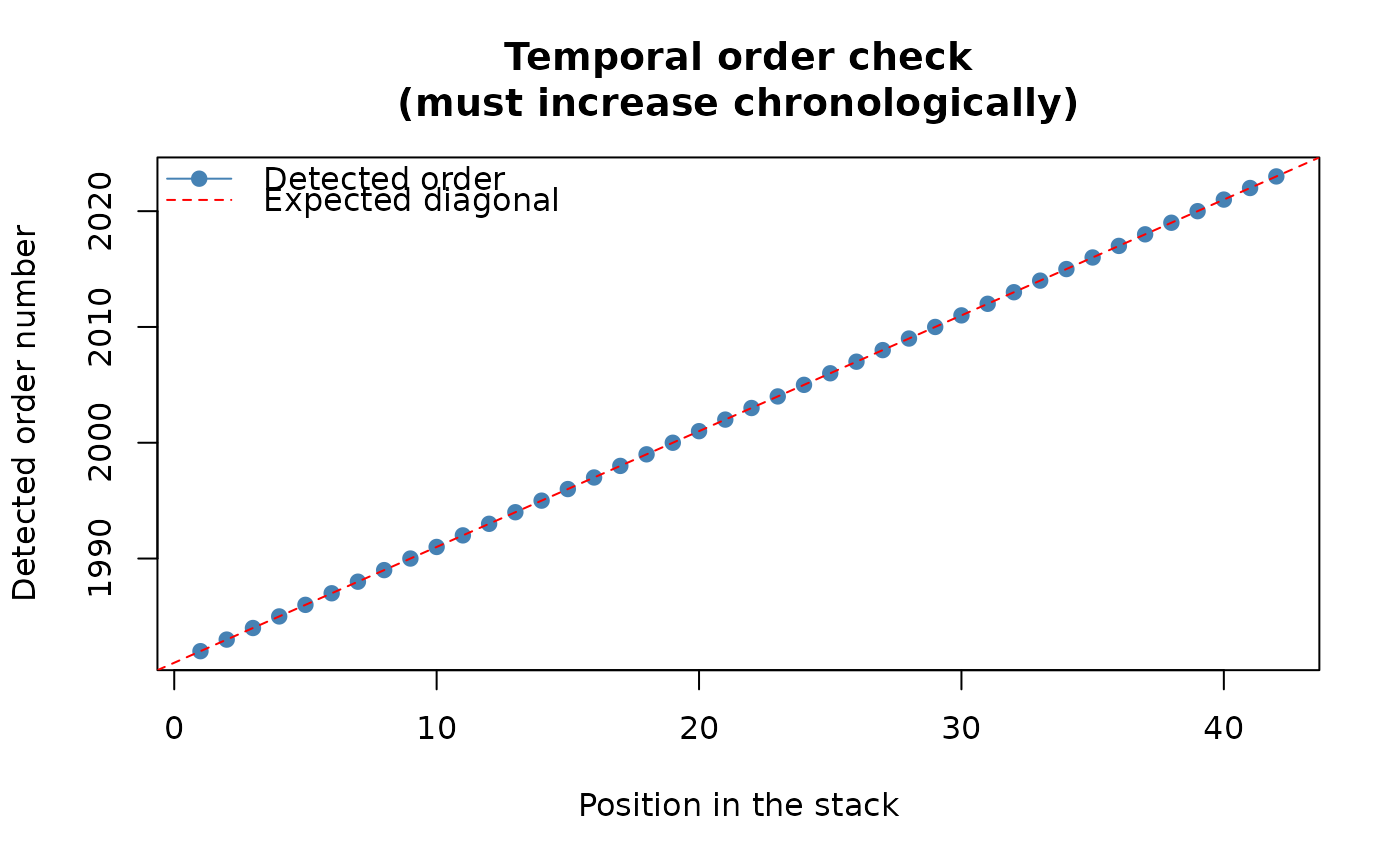#> Stack built: 42 layers, 146 x 338 cells.
#> >> [read_ordered_stack()] elapsed: 0.10 s

# Test every cell for a monotonic trend, borrowing strength from each
# cell's spatial neighbourhood (method = "CMK", the default).
trend <- trend_test(r, report = FALSE, verbose = FALSE)
trend
#> <Contextual Mann-Kendall (3x3) result>
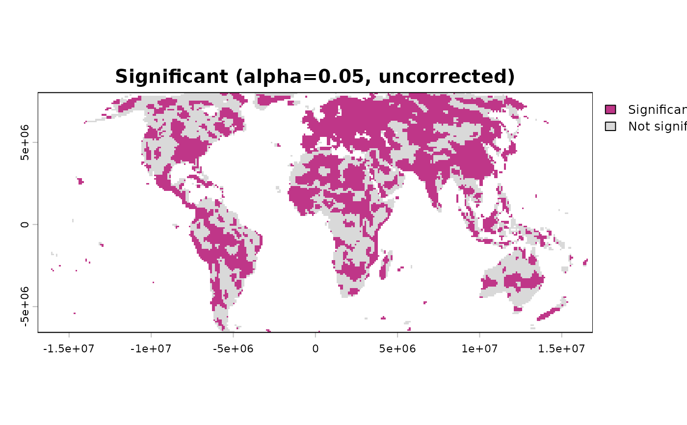
#> Cells tested: 15675 | significant at alpha=0.05 (uncorrected): 9004 (57.4%)
summary(trend)
#> Cells with complete time series: 15675
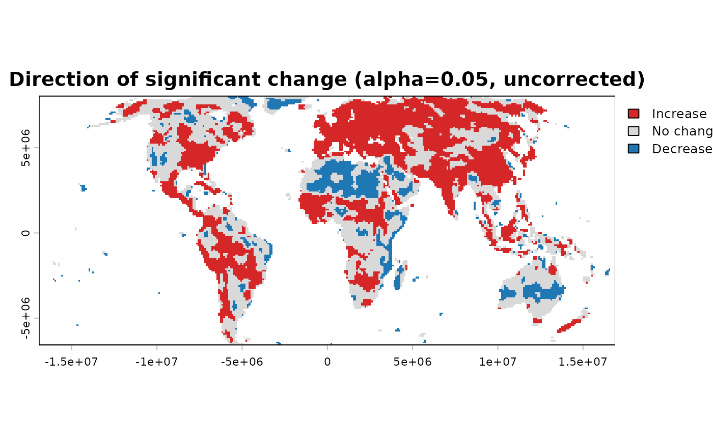
#> At alpha=0.05 -- increase: 7167 (45.7%) | decrease: 1837 (11.7%) | no change: 6671 (42.6%)

# Significance and direction, rather than the raw trend statistic.
plot(trend, panels = c("significance", "direction"))



# A larger odd window applies the CMK equations at a broader scale.
trend_5 <- trend_test(r, window_size = 5L, report = FALSE,
                       verbose = FALSE)
trend_5$window_size
#> [1] 5
# }