
Read and chronologically order a folder of raster files
Source:R/read_stack.R
read_ordered_stack.Rdlist.files() sorts alphabetically, not numerically: with file names
that lack leading zeros ("image1", ..., "image10"), "image10"
sorts before "image2" – the same problem regardless of whether the
numbering is a year, a time step, or any other sequential index.
Using that order silently invalidates a trend analysis with no
visible error anywhere in the code. This function instead extracts
an explicit ordering number from each file name and sorts
numerically by it, then prints and (optionally) plots a verification
of the detected order.
Usage
read_ordered_stack(
  dir = NULL,
  pattern = "\\.(tif|tiff|nc|grd|img|vrt|asc)$",
  order_regex = NULL,
  candidate_regex = c("year([0-9]+)", "_A([0-9]{4})", "(19[0-9]{2}|20[0-9]{2})",
    "([0-9]{4})", "([0-9]+)"),
  var = NULL,
  report = TRUE,
  verbose = TRUE,
  files = NULL,
  time = NULL,
  cycle_type = NULL,
  start = NULL,
  end = NULL,
  time_anchor = "centre"
)
Arguments
- dir
Character. Path to a folder containing one raster file per time step, all with the same extent, resolution, and CRS.
- pattern
Character. Regular expression used to list candidate files. The default matches common raster extensions:
.tif,.tiff,.nc,.grd,.img,.vrt, and.asc. Supply another expression for any additional format supported byterra::rast()/GDAL. The extension identifies candidate files; actual readability and compatible geometry are still validated when the stack is opened.- order_regex
Character or
NULL. A regular expression with a single capture group,"(...)", that extracts the ordering number from each file name – e.g."year([0-9]+)"extracts25from"year25.tif". IfNULL(default), several common patterns are tried automatically (year-like"year25", MODIS-style"_A2000065", a bare 4-digit year, or any run of digits) and the first one that extracts a unique number from every file is used. If none does, the function stops rather than silently falling back to alphabetical order.- candidate_regex
Character vector of patterns tried automatically when
order_regexisNULL. Most users should never need to modify this.- var
Character or
NULL. For NetCDF input only: variable name to read from each file if each file has more than one variable. LeaveNULLfor ordinary single-variable raster formats.- report
Logical. If
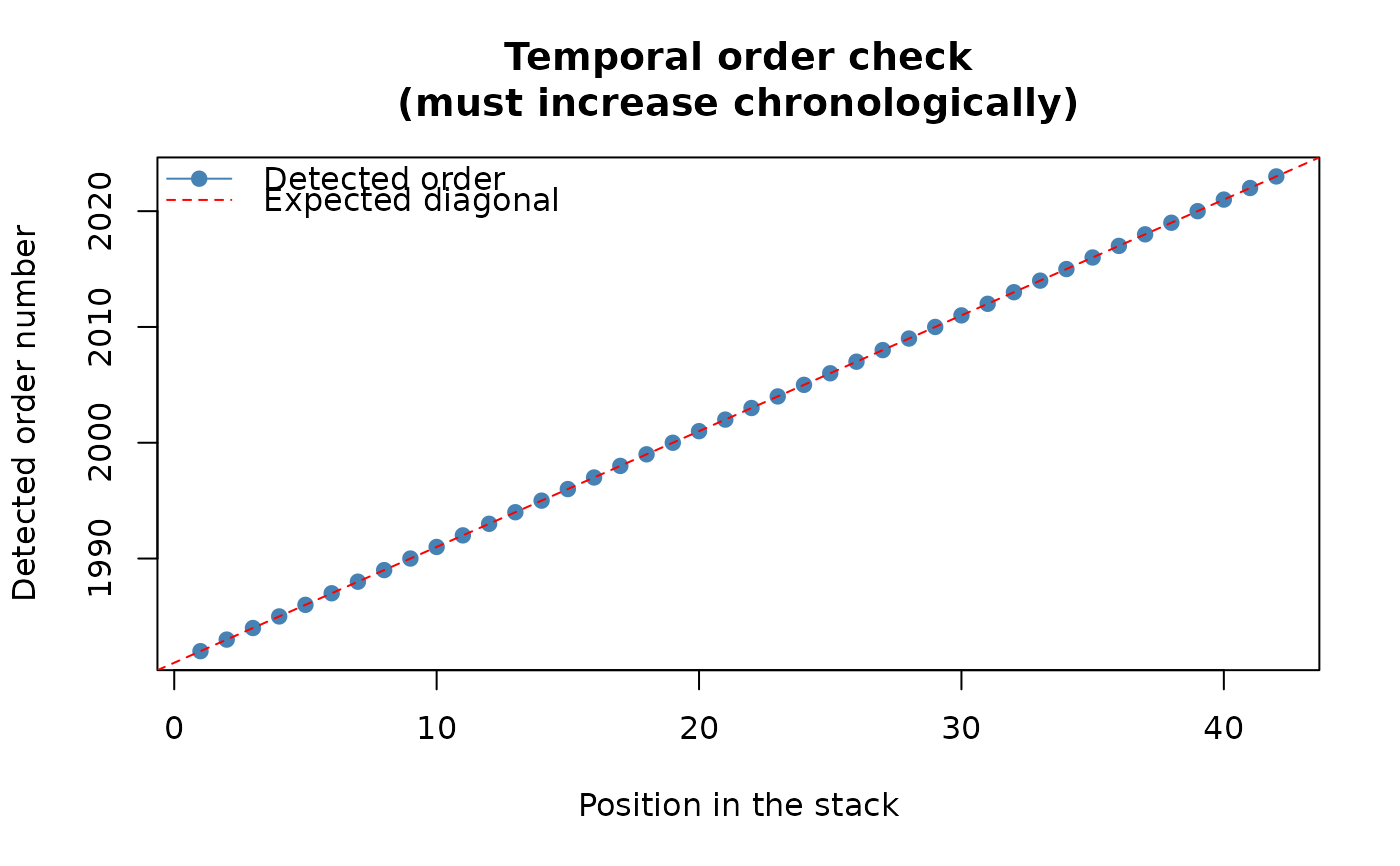
TRUE(default), draw a diagnostic plot of stack position vs. detected order number (a perfect diagonal line confirms correct ordering). Deviations from the diagonal immediately reveal files that would otherwise have been read in the wrong temporal order.- verbose
Logical. Print progress messages and elapsed time.
- files
Character vector of file paths, in the exact order you want them read as layers – no sorting of any kind is ever applied. Use instead of
dirwhenever automatic detection from file names is not reliable enough, which in practice means: whenever the series is not simply annual. The same numeric shape in a file name can mean genuinely different things across real datasets (e.g."19820102"is 2 January in some daily products, but the second half of January in PKU-GIMMS' own semimonthly convention) – automatic detection cannot resolve that safely, only declaring it explicitly can. Exactly one ofdirorfilesmust be supplied.- time
Optional. A
Date,POSIXct, or numeric vector, one value per layer, in the same order asfiles. Must be strictly increasing with no missing or duplicated values. The supplied file order and time vector are treated as authoritative – checked for internal consistency (right length, valid dates, correct order), not that you paired the right date with the right file; that correspondence remains your responsibility. Mutually exclusive withcycle_type. Requiresfiles.- cycle_type
Optional. One of
"annual","monthly","16-day","semimonthly","10-day","8-day","weekly", or"daily"– generates real calendar dates instead of you supplyingtimeyourself, for series that genuinely follow one of these conventions (see "Supported cycle types" above for the generative rule and real-product examples behind each). If your series does not follow one of these exact conventions, supplytimeexplicitly instead. Requiresfilesandstart.- start
Required with
cycle_type. A singleDatemarking the beginning of the first period. Must fall on a boundary valid for the declaredcycle_type(day 1 for"monthly"; day 1 or 16 for"semimonthly"; day 1, 11 or 21 for"10-day"; year-day 1, 17, 33, ..., 353 for"16-day"; year-day 1, 9, 17, ..., 361 for"8-day"; year-day 1, 8, ..., 358 for"weekly"; 1 January for"annual"; any date for"daily") – this checks that your own declaration is internally consistent, not that it matches your real product. If your product genuinely starts elsewhere, it does not follow thiscycle_typeconvention – supplyfiles+timeinstead.- end
Optional, only with
cycle_type. A singleDate, the final inclusive end of the last declared period. If omitted, the number of layers found infilesdetermines how many dates are generated fromstartonward. If supplied, the calendar expected betweenstartandendis built first, and the number of layers found must match that expected count exactly – this is what detects an incomplete series (e.g. a declared full year missing one month's file), which omittingendcannot catch on its own.- time_anchor
One of
"start","centre"(default), or"end". Only applicable withcycle_type = "monthly","semimonthly","10-day","16-day","8-day"or"weekly". Annual layers are always dated 1 January; daily layers use their own date. Do not supplytime_anchorfor these two conventions. Controls which point within each period's own date range is assigned as that layer's date – irrelevant for MK/CMK (rank-based), but affects the numeric time values OLS/MMK use directly. For a period with an even number of days,"centre"deterministically picks the earlier of the two central days.
Value
A terra::SpatRaster with one layer per time step, ordered
chronologically – one layer per input file for ordinary single-layer
formats (the typical case), but a single input file can contribute
more than one layer for multi-layer formats (e.g. a NetCDF file with
several time steps of its own; files and the explicit modes fully
support this, tracking which layers came from which file for the
verbose order-check table). Layer names are taken from the
(de-duplicated) file names, and temporal order is stored as proper
time metadata (terra::time(result)) rather than discarded after
the verification step above – used, for instance, as the default
t in inspect_ts_cell(), and by any future function in this
package requiring explicit time coordinates.
Details
Works with raster formats readable by terra::rast(), subject to the
GDAL drivers available in the user's terra installation. The default
pattern covers common GeoTIFF, NetCDF, native raster, ERDAS Imagine,
virtual raster and ASCII-grid extensions; other supported formats can
be selected through pattern. Each file must represent one time step.
For a single multi-temporal NetCDF file instead, use
read_netcdf_stack().
Why this matters more than it looks: a trend analysis assumes
that successive raster layers represent the true chronological
sequence. If the temporal order is wrong, every subsequent
statistical result becomes invalid even though the analysis
completes without any error – there is nothing in a Mann-Kendall
test's own output that could reveal a shuffled input series. Unlike
generic file readers, this function deliberately refuses to proceed
when the temporal order cannot be established unambiguously, rather
than silently reverting to alphabetical file names. This same
philosophy – surface a silent risk rather than let it pass
unnoticed – recurs throughout this package: multiple-testing
correction (fdr_correction()), the spatial-autocorrelation
diagnostic behind it (spatial_autocorrelation()), and the
monotonic-trend-only assumption checked informally in "Monotonic
trends only" sections elsewhere (trend_test(),
slope_estimator()) are the same instinct applied to different
risks.
This function does not use list.files()'s own ordering, does not
attempt to parse arbitrary or ambiguous date formats, and does not
guess when no candidate pattern extracts a unique number from every
file – it stops instead, on the view that it is better to stop than
to silently analyse the wrong chronology.
Function type: Data import function – builds the ordered
SpatRaster expected by the analytical functions. It performs no
statistical inference.
Methodological details
Temporal ordering
Ordering is derived from explicit numeric labels in file names, never from alphabetical order. Ambiguous, duplicated, or incomplete labels stop the import rather than trigger an undocumented fallback.
Explicit declaration (files, time, cycle_type)
Automatic detection above only extracts one ordering number per file
name, which is reliable for genuinely annual series but not for finer
cadences: the same numeric shape in a file name can mean genuinely
different things across real datasets – "19820102" is 2 January in
some daily products, but the second half of January under PKU-GIMMS
NDVI's own semimonthly convention. files (an explicit, already
correctly ordered vector) sidesteps this by never interpreting file
names at all; combined with time (fully explicit dates) or
cycle_type (a named calendar convention) it is recommended whenever
the series is not simply annual.
Supported cycle types
Eight unambiguous calendar conventions, all built with genuine calendar
arithmetic (leap years included) rather than naive interval division.
Fixed compositing intervals that do not follow one of these exact
conventions (e.g. a genuinely continuous 8-day or 16-day interval) are
out of scope for cycle_type – supply time explicitly instead.
"annual"One date per year, 1 January. 1 sample/year. E.g. the bundled
example_data("vhp_ndvi")dataset itself."monthly"One period per calendar month, beginning on the 1st. 12 samples/year. E.g. CRU TS, TerraClimate, ERA5 monthly means.
"16-day"23 fixed periods per year, resetting every 1 January (never continuing across a year boundary), starting on year-day 1, 17, 33, ..., 353 – the last period of the year is shorter (13 or 14 days) to fit within the calendar year. Matches MODIS' own 16-day compositing convention (e.g. MOD13Q1), verified directly against real product file names.
"semimonthly"Two periods per calendar month, beginning on the 1st and the 16th. 24 samples/year. Matches PKU-GIMMS NDVI's own "half-month" convention – not the same cadence as a continuous 14-day interval.
"10-day"Three calendar periods per month, starting on the 1st, 11th and 21st (the last one running to the end of the month, so its own length varies: 8 to 11 days). 36 samples/year. The standard "dekad" convention, e.g. SPOT-VEGETATION and several FEWS NET agricultural products – not a continuous 10-day interval, which would not align with month boundaries and would give a different total (37, not 36).
"8-day"46 fixed periods per year, resetting every 1 January, starting on year-day 1, 9, 17, ..., 361 – the last period of the year is shorter, capturing the remainder. Matches MODIS' own 8-day compositing convention (e.g. MCD15A2H, the LAI/FPAR product).
"weekly"52 fixed, complete 7-day periods per year (Earth Trends Modeler's own number), starting on year-day 1, 8, ..., 358 – unlike
"8-day"/"16-day", the final one or two days of the year belong to no period and are skipped straight into next year's first period, rather than forming a shorter final period."daily"One date per real calendar day, including 29 February in leap years. 365 or 366 samples/year – the only one of these eight where the yearly total itself changes with leap years (the other seven keep a fixed count per year; only the exact date of late-period boundaries shifts). E.g. ERA5, CHIRPS daily precipitation.
"weekly"'s own remainder-discarding convention (unlike the other
fixed-interval types here) is not this function's own inconsistency
– it follows Earth Trends Modeler's own table exactly for each
named type individually, and that table is not internally
consistent on this specific point across its own listed
conventions.
Monthly or seasonal data
This function only orders layers chronologically – it does not know
or care whether the data has a seasonal cycle (e.g. monthly values with
an annual signal). If it does, deseasonalise with compute_anomalies()
before passing the result to trend_test(),
slope_estimator(), or workflow_tst(), all of which assume a
monotonic trend,
not a periodic one. Ordering and deseasonalisation solve different
problems.
Limitations
Files must share compatible raster geometry and each file must
represent one time step. Automatic detection deliberately does not
attempt to infer arbitrary calendar formats that are not captured by
the supplied or candidate regular expressions – use files with
time or cycle_type for those cases instead of expecting automatic
detection to guess correctly.
Quality assurance
Tests cover year and year-month filename parsing, chronological
ordering, duplicate and ambiguous labels, mixed geometries, variable
selection, preserved terra geometry/time metadata, and informative
failures for empty or invalid inputs. See ?sptrends for the
package-wide release-check protocol.
See also
Other Data import functions:
read_netcdf_stack()
Examples
# \donttest{
# The bundled dataset contains one real NDVI GeoTIFF per year.
s <- read_ordered_stack(example_data("vhp_ndvi"))
#> Temporal order auto-detected with pattern '(19[0-9]{2}|20[0-9]{2})'.
#> Automatic mode: order detected from file names. For higher reliability -- especially if the series is not annual -- supplying 'files' explicitly (with 'time' or 'cycle_type') is recommended. See ?read_ordered_stack.
#> Temporal order verification (mandatory, cannot be skipped):
#> stack_position detected_number file
#> 1 1982 VHP_SMN_annual_ndvi_1982.tif
#> 2 1983 VHP_SMN_annual_ndvi_1983.tif
#> 3 1984 VHP_SMN_annual_ndvi_1984.tif
#> 4 1985 VHP_SMN_annual_ndvi_1985.tif
#> 5 1986 VHP_SMN_annual_ndvi_1986.tif
#> 6 1987 VHP_SMN_annual_ndvi_1987.tif
#> 7 1988 VHP_SMN_annual_ndvi_1988.tif
#> 8 1989 VHP_SMN_annual_ndvi_1989.tif
#> 9 1990 VHP_SMN_annual_ndvi_1990.tif
#> 10 1991 VHP_SMN_annual_ndvi_1991.tif
#> 11 1992 VHP_SMN_annual_ndvi_1992.tif
#> 12 1993 VHP_SMN_annual_ndvi_1993.tif
#> 13 1994 VHP_SMN_annual_ndvi_1994.tif
#> 14 1995 VHP_SMN_annual_ndvi_1995.tif
#> 15 1996 VHP_SMN_annual_ndvi_1996.tif
#> 16 1997 VHP_SMN_annual_ndvi_1997.tif
#> 17 1998 VHP_SMN_annual_ndvi_1998.tif
#> 18 1999 VHP_SMN_annual_ndvi_1999.tif
#> 19 2000 VHP_SMN_annual_ndvi_2000.tif
#> 20 2001 VHP_SMN_annual_ndvi_2001.tif
#> 21 2002 VHP_SMN_annual_ndvi_2002.tif
#> 22 2003 VHP_SMN_annual_ndvi_2003.tif
#> 23 2004 VHP_SMN_annual_ndvi_2004.tif
#> 24 2005 VHP_SMN_annual_ndvi_2005.tif
#> 25 2006 VHP_SMN_annual_ndvi_2006.tif
#> 26 2007 VHP_SMN_annual_ndvi_2007.tif
#> 27 2008 VHP_SMN_annual_ndvi_2008.tif
#> 28 2009 VHP_SMN_annual_ndvi_2009.tif
#> 29 2010 VHP_SMN_annual_ndvi_2010.tif
#> 30 2011 VHP_SMN_annual_ndvi_2011.tif
#> 31 2012 VHP_SMN_annual_ndvi_2012.tif
#> 32 2013 VHP_SMN_annual_ndvi_2013.tif
#> 33 2014 VHP_SMN_annual_ndvi_2014.tif
#> 34 2015 VHP_SMN_annual_ndvi_2015.tif
#> 35 2016 VHP_SMN_annual_ndvi_2016.tif
#> 36 2017 VHP_SMN_annual_ndvi_2017.tif
#> 37 2018 VHP_SMN_annual_ndvi_2018.tif
#> 38 2019 VHP_SMN_annual_ndvi_2019.tif
#> 39 2020 VHP_SMN_annual_ndvi_2020.tif
#> 40 2021 VHP_SMN_annual_ndvi_2021.tif
#> 41 2022 VHP_SMN_annual_ndvi_2022.tif
#> 42 2023 VHP_SMN_annual_ndvi_2023.tif
 #> Stack built: 42 layers, 146 x 338 cells.
#> >> [read_ordered_stack()] elapsed: 0.11 s
terra::nlyr(s)
#> [1] 42
terra::time(s, "years")
#> [1] 1982 1983 1984 1985 1986 1987 1988 1989 1990 1991 1992 1993 1994 1995 1996
#> [16] 1997 1998 1999 2000 2001 2002 2003 2004 2005 2006 2007 2008 2009 2010 2011
#> [31] 2012 2013 2014 2015 2016 2017 2018 2019 2020 2021 2022 2023
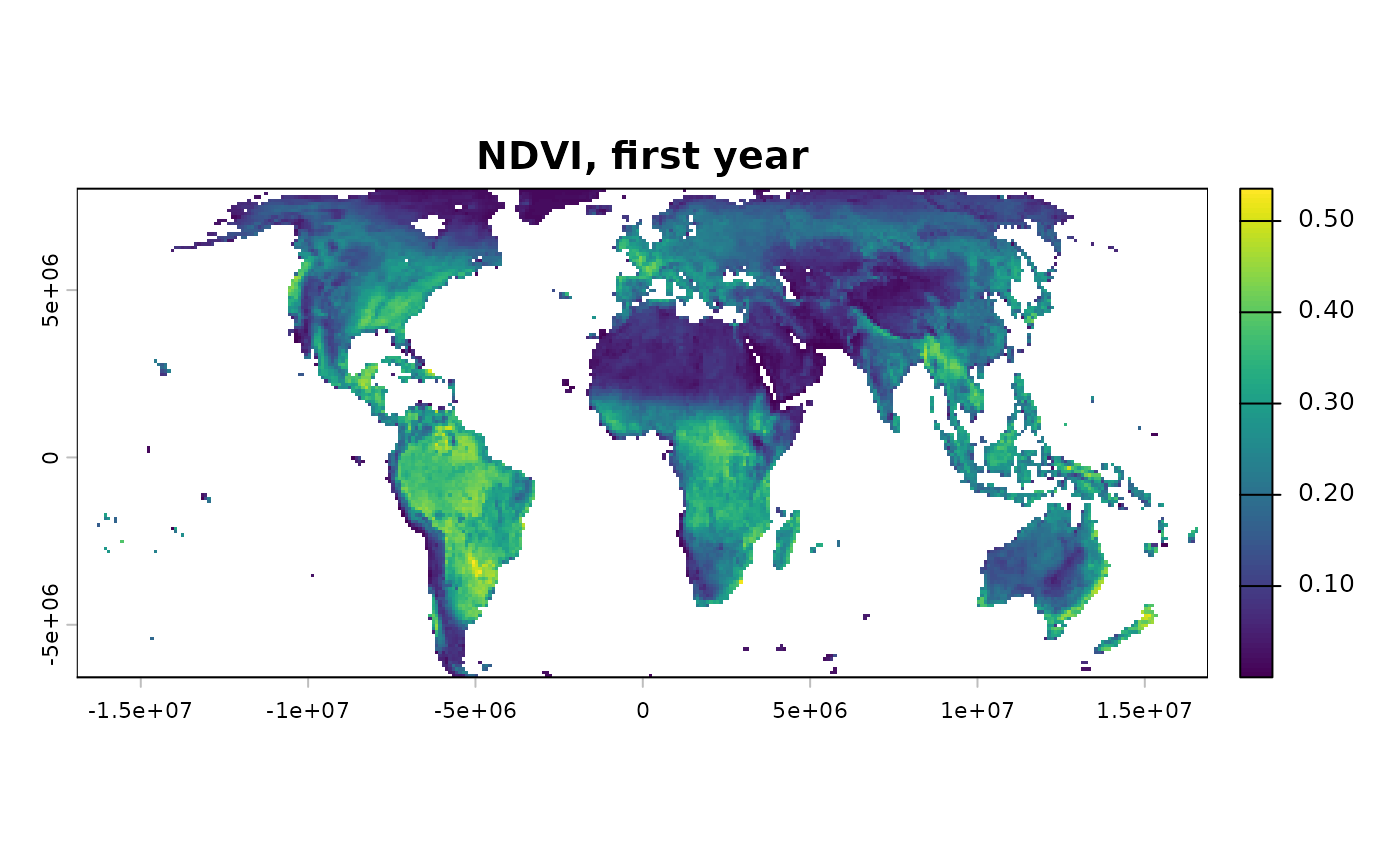
terra::plot(s[[1]], main = "NDVI, first year")
#> Stack built: 42 layers, 146 x 338 cells.
#> >> [read_ordered_stack()] elapsed: 0.11 s
terra::nlyr(s)
#> [1] 42
terra::time(s, "years")
#> [1] 1982 1983 1984 1985 1986 1987 1988 1989 1990 1991 1992 1993 1994 1995 1996
#> [16] 1997 1998 1999 2000 2001 2002 2003 2004 2005 2006 2007 2008 2009 2010 2011
#> [31] 2012 2013 2014 2015 2016 2017 2018 2019 2020 2021 2022 2023
terra::plot(s[[1]], main = "NDVI, first year")
 # }
# }