Remove the seasonal cycle from raster time series

Monotonic trend tests assume that the input series does not contain a regular periodic component – the ranking of observations should primarily reflect long-term change, not where in the year a value falls. When a seasonal cycle is present (e.g. monthly means over many years), that cycle itself dominates the ranking and can obscure or distort the monotonic signal a trend test is looking for.

Usage

compute_anomalies(
  x,
  cycle = 12,
  cycle_type = NULL,
  start_position = 1,
  standardise = FALSE,
  verbose = TRUE
)

Arguments

x: A terra::SpatRaster with nlyr(x) a multiple of cycle (or not – a partial final cycle is allowed, but its climatology mean will be based on fewer years for those positions).
cycle: Integer. Length of the seasonal cycle in layers – e.g. 12 for monthly data with an annual cycle (the default), 4 for quarterly/seasonal data. A daily annual cycle requires a consistent calendar with the same positions in every year. Ignored if cycle_type is supplied.
cycle_type: Optional named shortcut for cycle, using the same vocabulary as read_ordered_stack()'s own cycle_type (see ?read_ordered_stack, "Supported cycle types"): "monthly" (12), "16-day" (23), "semimonthly" (24), "10-day" (36), "8-day" (46), or "weekly" (52). "annual" and "daily" are deliberately not included – see "Methodological details" below. NULL (default) uses the numeric cycle instead.
start_position: Integer in [1, cycle]. Cycle position of the stack's first layer. Default 1 (the first layer is the first position of its cycle, e.g. January for monthly data). Set this when a series starts mid-cycle – e.g. start_position = 8 for monthly data beginning in August, so the climatology aligns layers to their true calendar position instead of assuming the stack starts at the beginning of a cycle.
standardise: Logical. If FALSE (default), returns raw anomalies (x - climatology_mean), in the original units – preserves the variable's own physical units, and is the more common choice when that is what downstream reporting needs. If TRUE, also divides by the per-cycle-position standard deviation (z-scores: (x - climatology_mean) / climatology_sd), making the anomaly magnitude comparable across cycle positions that have very different natural variability (e.g. winter vs. summer temperature variance) – useful specifically when comparing or combining anomalies across cycle positions whose natural spread differs. Cycle positions with zero standard deviation (constant across all years) get NA anomalies rather than a division by zero.
verbose: Logical. Print progress messages and elapsed time.

Value

Returns a list with:

anomalies: A SpatRaster, same number of layers as x – raw or standardised depending on standardise.
climatology: A SpatRaster with cycle layers (the mean field for each position in the cycle), ordered from position 1 to cycle, regardless of start_position.
climatology_sd: Only if standardise = TRUE: a SpatRaster with cycle layers (the standard deviation field for each position in the cycle), in the same order as climatology.

A plain list, not a classed "sptrends" object – unlike prewhiten() or trend_test(), this function's output is typically fed straight into the next preprocessing or inferential step rather than inspected on its own via print()/summary()/ plot().

Details

This function removes that cycle by computing the mean value at each position within it (e.g. the mean of all Januaries, all Februaries, ...) – the climatology – and subtracting it from every layer at that position, leaving an anomaly series: successive observations that are directly comparable to one another, with the seasonal pattern removed. This is appropriate input for trend_test() or prewhiten(), both of which assume no periodic component – in a typical workflow, this function is applied first, before prewhiten(), since prewhitening's own AR(1) model assumes the series it receives has no remaining seasonal structure of its own.

Function type: Preprocessing function – prepares seasonal raster time series before prewhitening or trend analysis. It is not itself a trend test or slope estimator.

Typical use

seasonal raster time series
    |
compute_anomalies()
    |
anomaly time series (`result$anomalies`)
    |
prewhiten(), trend_test(), or workflow_trends()

Apply this step only when x contains a recurring seasonal cycle. workflow_tst() and workflow_trends() start from prewhitening or trend analysis, so pass result$anomalies, rather than the original seasonal series, when deseasonalisation is required.

Methodological details

How it works

A simple mean per cycle position, over the whole series – not a moving climatology, a LOESS-smoothed seasonal curve, or a spline fit. This is deliberately the simplest well-defined choice, not a limitation to work around: for the purpose of removing a fixed seasonal pattern before a monotonic-trend test, a fixed per-position mean is sufficient, and a more elaborate seasonal model would add complexity without changing what this function is for.

Statistical assumptions

The seasonal cycle has a known, fixed length and corresponding cycle positions are comparable across repetitions. The estimated fixed climatology is assumed to represent the recurring component that should be removed before later analysis.

Limitations

This function does not detrend the series in any other sense: the climatology is computed directly over the raw values at each cycle position, so a strong underlying trend is already partly absorbed into the climatology mean itself (e.g. if summers have been getting warmer throughout the record, the "mean summer" climatology reflects an average across that warming, not any single year's summer). This is expected, not a defect – it is the trend test applied afterwards that isolates the trend itself; this function's only job is removing the periodic component. Likewise, a genuine regime shift (an abrupt, one-time change in the seasonal pattern partway through the series, as opposed to a gradual trend) would show up mixed into the climatology rather than being detected as such – this function has no mechanism to distinguish a regime shift from ordinary seasonal variability; that is a different kind of question from the one it answers.

Why cycle_type excludes "annual" and "daily"

"annual" would translate to cycle = 1, which this function always rejects immediately afterwards – an annual series has no sub-annual cycle to remove in the first place, so there is nothing for this function to do with it. "daily" would use a fixed cycle = 365 based on cycle position alone; this function does not use the dates in terra::time(x). Keeping leap days would misalign the climatology for the rest of the series (day 366 would be paired with the cycle position that day 1 of the following year would otherwise occupy). Use a numeric cycle only when each cycle has the same number of comparable positions. Reading daily dates with read_ordered_stack() does not change this positional grouping rule.

Quality assurance

Tests verify monthly and arbitrary-cycle climatologies against direct calculations, centred and standardised anomalies, layer names, retained geometry, missing values, zero-variance cycles, non-default starting positions (including partial cycles), and invalid inputs. Workflow tests confirm that anomaly outputs remain compatible with later preprocessing and trend stages. See ?sptrends for the common release-check protocol.

References

General references for the anomaly/standardisation concept (removing a periodic mean, optionally scaling by its standard deviation) – not a single named method with one original paper, but a standard technique in climatology and atmospheric science:

Wilks, D.S. (2019) Statistical Methods in the Atmospheric Sciences (4th edn). Elsevier/Academic Press. No DOI available (book).
Mather, P.M. (1999) Computer Processing of Remotely-Sensed Images. John Wiley and Sons.

Examples

# The bundled NDVI series is annual and therefore has no subannual
# climatological cycle to remove.
r <- read_ordered_stack(example_data("vhp_ndvi"))
#> Temporal order auto-detected with pattern '(19[0-9]{2}|20[0-9]{2})'.
#> Automatic mode: order detected from file names. For higher reliability -- especially if the series is not annual -- supplying 'files' explicitly (with 'time' or 'cycle_type') is recommended. See ?read_ordered_stack.
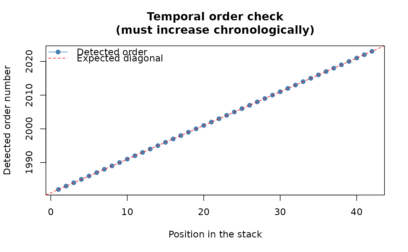
#> Temporal order verification (mandatory, cannot be skipped):
#>  stack_position detected_number                         file
#>               1            1982 VHP_SMN_annual_ndvi_1982.tif
#>               2            1983 VHP_SMN_annual_ndvi_1983.tif
#>               3            1984 VHP_SMN_annual_ndvi_1984.tif
#>               4            1985 VHP_SMN_annual_ndvi_1985.tif
#>               5            1986 VHP_SMN_annual_ndvi_1986.tif
#>               6            1987 VHP_SMN_annual_ndvi_1987.tif
#>               7            1988 VHP_SMN_annual_ndvi_1988.tif
#>               8            1989 VHP_SMN_annual_ndvi_1989.tif
#>               9            1990 VHP_SMN_annual_ndvi_1990.tif
#>              10            1991 VHP_SMN_annual_ndvi_1991.tif
#>              11            1992 VHP_SMN_annual_ndvi_1992.tif
#>              12            1993 VHP_SMN_annual_ndvi_1993.tif
#>              13            1994 VHP_SMN_annual_ndvi_1994.tif
#>              14            1995 VHP_SMN_annual_ndvi_1995.tif
#>              15            1996 VHP_SMN_annual_ndvi_1996.tif
#>              16            1997 VHP_SMN_annual_ndvi_1997.tif
#>              17            1998 VHP_SMN_annual_ndvi_1998.tif
#>              18            1999 VHP_SMN_annual_ndvi_1999.tif
#>              19            2000 VHP_SMN_annual_ndvi_2000.tif
#>              20            2001 VHP_SMN_annual_ndvi_2001.tif
#>              21            2002 VHP_SMN_annual_ndvi_2002.tif
#>              22            2003 VHP_SMN_annual_ndvi_2003.tif
#>              23            2004 VHP_SMN_annual_ndvi_2004.tif
#>              24            2005 VHP_SMN_annual_ndvi_2005.tif
#>              25            2006 VHP_SMN_annual_ndvi_2006.tif
#>              26            2007 VHP_SMN_annual_ndvi_2007.tif
#>              27            2008 VHP_SMN_annual_ndvi_2008.tif
#>              28            2009 VHP_SMN_annual_ndvi_2009.tif
#>              29            2010 VHP_SMN_annual_ndvi_2010.tif
#>              30            2011 VHP_SMN_annual_ndvi_2011.tif
#>              31            2012 VHP_SMN_annual_ndvi_2012.tif
#>              32            2013 VHP_SMN_annual_ndvi_2013.tif
#>              33            2014 VHP_SMN_annual_ndvi_2014.tif
#>              34            2015 VHP_SMN_annual_ndvi_2015.tif
#>              35            2016 VHP_SMN_annual_ndvi_2016.tif
#>              36            2017 VHP_SMN_annual_ndvi_2017.tif
#>              37            2018 VHP_SMN_annual_ndvi_2018.tif
#>              38            2019 VHP_SMN_annual_ndvi_2019.tif
#>              39            2020 VHP_SMN_annual_ndvi_2020.tif
#>              40            2021 VHP_SMN_annual_ndvi_2021.tif
#>              41            2022 VHP_SMN_annual_ndvi_2022.tif
#>              42            2023 VHP_SMN_annual_ndvi_2023.tif

#> Stack built: 42 layers, 146 x 338 cells.
#> >> [read_ordered_stack()] elapsed: 0.35 s
terra::nlyr(r)
#> [1] 42
# Apply compute_anomalies() only to real observations with a genuine
# cycle, for example cycle = 12 for monthly data.