AR(1) prewhitening of raster time series

Removes temporal (serial) autocorrelation from each cell's time series while preserving its linear trend, using one of four published methods (see the method argument below for the choice). The default, "TFPW_WS": for each cell, fit an OLS trend, compute the Durbin-Watson statistic of the residuals, and – only for cells where DW indicates relevant serial autocorrelation – iteratively estimate the AR(1) coefficient rho and apply a trend-preserving transformation (with a Prais-Winsten correction for the first observation). Cells that pass the DW check are left untouched.

Usage

prewhiten(
  x,
  method = c("TFPW_WS", "TFPW_Y", "TFPW_Z", "VCTFPW"),
  t,
  dw_low = 1.4,
  dw_high = 2.6,
  dw_method = c("threshold", "test"),
  dw_inconclusive = c("conservative", "power"),
  eps = 1e-04,
  itmax = 20,
  refit_method = c("OLS", "TS"),
  report = TRUE,
  verbose = TRUE
)

Arguments

x

A terra::SpatRaster; each layer is one time step, in increasing chronological order.

method

Which prewhitening method to use, sharing one interface between four related procedures (see "Methodological details" below for the full comparison and citations).

"TFPW_WS" (default; TFPW-WS, also seen as "Wang-Swail prewhitening" in the literature):

Description: the selective AR(1) prewhitening described above, gated by a Durbin-Watson diagnostic.
Characteristics: only cells that need it get modified; rho is estimated on the raw trend residuals.
Advantage: avoids the power loss of prewhitening cells that already behave like white noise (see "Statistical rationale" above).

"TFPW_Y" (TFPW-Y, also seen simply as "TFPW" – this is the best-known formulation of trend-free prewhitening in the literature):

Description: trend-free pre-whitening (Yue, Pilon, Cavadias, 2002).
Characteristics: estimates a Theil-Sen slope per cell first, removes it, estimates lag-1 autocorrelation on the detrended residuals (not the raw series, which would over-estimate rho when a real trend is present), prewhitens those residuals, and adds the slope back; every valid cell is processed unconditionally, there is no DW gate.
Advantage: a single, simple rule applied uniformly, with no threshold or test choice to make.

"TFPW_Z" (TFPW-Z here – not a universally established acronym in the literature the way the others are, so defined explicitly wherever used):

Description: Zhang, Vincent, Hogg and Niitsoo (2000), as later refined into TFPW_WS above – this method is the earlier, unrefined form the same iterative mechanism (see "Implementation notes" above) is traced against and mirrors.
Characteristics: identical iteration to TFPW_WS, but with no Durbin-Watson gate – every valid cell is processed unconditionally, matching zyp::zyp.TFPW_Z()'s own published behaviour.
Advantage: no gating decision to make, at the same cost TFPW_Y has for the same reason.

"VCTFPW" (VCTFPW):

Description: variance-corrected trend-free prewhitening (Wang, Chen, Becker and Liu, 2015).
Characteristics: removes a Sen slope, estimates lag-1 autocorrelation on the detrended residuals and applies the published transformation only where that autocorrelation is significant at the two-sided 95% level. It then applies the published variance-ratio correction and corrects the restored slope for positive autocorrelation. Cells that do not cross the gate retain their original series.
Advantage: addresses a specific, published criticism of simpler trend-free methods – their own reduced variance biases the slope and its significance – at the cost of a substantially more involved procedure.

Comparison: TFPW_WS uses a Durbin-Watson gate, TFPW_Z and TFPW_Y process every valid cell unconditionally, and VCTFPW uses its published 95% lag-1-autocorrelation gate before applying its variance and slope corrections. See "Methodological details" above for the full citations and practical implications of each.

t

Numeric vector of time points, one per layer. Defaults to 1:nlyr(x). Irregular spacing is supported, but values must be finite, unique and strictly increasing.

dw_low, dw_high

Only used when method = "TFPW_WS". Fixed Durbin-Watson gate thresholds, used only when dw_method = "threshold".

dw_method

Only used when method = "TFPW_WS". "threshold" (default): use the fixed dw_low/dw_high cutoffs. "test": use the formal Durbin-Watson test with critical values (dL, dU) tabulated for the actual sample size, at the 5% level.

dw_inconclusive

Only used when method = "TFPW_WS" and dw_method = "test". The classic DW test has an inconclusive zone (dL <= DW <= dU) where it cannot decide – this is not the same as "autocorrelation present". "conservative" (default) prewhitens that zone too (favours not leaving autocorrelation uncorrected); "power" prewhitens only when the test actually rejects H0 (DW < dL), favouring statistical power downstream. Neither is "the correct" choice in absolute terms.

eps

Only used when method = "TFPW_WS" or "TFPW_Z". Convergence threshold for the iterative estimation of rho.

itmax

Only used when method = "TFPW_WS" or "TFPW_Z". Maximum number of iterations. TerrSet's own Earth Trends Modeler, which implements this same method, caps this at 5 "to avoid the rare cases that fail to converge" (its own documentation's wording) – sptrends uses a higher default (20) instead, relying on Clamped (see "Value" below) to flag a cell whose own iteration did not settle within that budget, rather than capping the budget itself as tightly as TerrSet does.

refit_method

Only used when method = "TFPW_WS" or "TFPW_Z". Which slope estimator re-fits the trend at each iteration, before removing it to isolate the residual autocorrelation for the next rho estimate: "OLS" (default, matching this function's own behaviour in earlier package versions) or "TS" (Theil-Sen, matching the original iterative procedure as multiple independent sources describe Wang and Swail (2001) actually publishing it – see "Implementation notes" below for the specific evidence and why the default was not simply changed to match it outright). "TS"'s own robustness to outliers can matter specifically for a cell whose iteration is already unstable (see Clamped below): an extreme value in one iteration's own transformed series distorts an "OLS" refit more than a "TS" one, which can itself feed into a worse rho estimate the following iteration. Comparing both directly on a specific Clamped = 1 cell, the same way comparing TFPW_WS against TFPW_Y is already recommended for that case (see "Value" below), is worth doing before trusting either estimate in isolation.

report

Logical. If TRUE (default), automatically print a summary and draw diagnostic histograms and maps after computing (which functions, exactly, depends on method – see "Value" below). Set to FALSE for programmatic use (e.g. inside a loop, or when called from workflow_tst()) where you don't want console output or plots as a side effect.

verbose

Logical. Print progress messages and elapsed time.

Value

Returns a list of class "prewhiten", with:

series: A SpatRaster. For method = "TFPW_WS": same structure as x, with prewhitened cells replaced and the rest unchanged; layer names get a "_prewhitened" suffix. For method = "TFPW_Y": one fewer layer than x (the classic Yue-Pilon transform loses the first time step to lag-1 differencing); every valid cell is prewhitened, with its Theil-Sen trend preserved; layer names come from x's own layers 2 through n, with a "_prewhitened" suffix. For method = "TFPW_Z": the same number of layers as x; every valid cell enters the same iterative transformation used by TFPW_WS, but without the Durbin-Watson gate. For method = "VCTFPW": the same number of layers as x; significantly autocorrelated cells contain the published VCTFPW transformation and other valid cells remain unchanged.
diagnostics: A SpatRaster. For method = "TFPW_WS": 4 layers, DW_initial, Rho, Modified (0/1), and Clamped (0/1) – Clamped is 1 for a gated cell whose iterative rho estimate hit the +-1 stability bound (see "Implementation notes" below) at any point during the iteration, even if a later iteration's own rho - rho_old difference happened to fall under eps immediately afterwards, since a Rho reaching that bound reflects the bound itself, not necessarily a precise, well-converged estimate. A clamped cell is deliberately left uncorrected (series keeps its original observed values there, Modified is 0 for it) rather than transformed using that unreliable rho: the correction divides by (1 - rho), so at rho = 0.99 the residuals would be multiplied by 100 – an extreme, disproportionate transform for what was, underneath, an unstable rather than a trustworthy estimate. Rho still records the clamped value itself, so the reason a cell went uncorrected remains visible in the diagnostics rather than indistinguishable from a cell that never needed correcting in the first place. Reachable via summary()/plot() as prewhiten_summary()/prewhiten_histograms()/ prewhiten_maps(). For method = "TFPW_Y": 2 layers, Beta_TheilSen (the slope removed and restored) and Rho (lag-1 autocorrelation of the detrended residuals); reachable via internal reporting functions specific to this method, not the TFPW_WS ones above (their structure differs – there is no DW gate, Modified, or Clamped field for TFPW_Y, which does not iterate to estimate rho and so cannot hit this same failure mode – precisely why comparing both methods on the same data is worth doing for a cell flagged Clamped = 1, rather than trusting either one in isolation: agreement between them is reassuring, and disagreement is itself informative about how sensitive that cell's own result is to the prewhitening method chosen.). For method = "TFPW_Z": the same 4 layers as TFPW_WS, but DW_initial is NA because this method has no Durbin-Watson gate; every valid cell enters the iteration, while Modified and Clamped retain the meanings described above. For method = "VCTFPW": 3 layers, Rho (lag-1 autocorrelation of the detrended series), Beta_corrected, and Modified (0/1, indicating whether the 95% autocorrelation gate was crossed).
method: The selected method, recorded as one of "TFPW_WS", "TFPW_Y", "TFPW_Z", or "VCTFPW".

Details

Function type: Preprocessing function – prepares the raw raster time series before trend estimation or significance testing (see compute_anomalies() for the other preprocessing step this package offers). Not one of the core trend-analysis pillars itself. This function typically precedes trend estimation (trend_test()) and slope estimation (slope_estimator()) within the standard sptrends workflow.

Typical use

This function is the preprocessing step between reading data and testing it for a trend: read_ordered_stack()/read_netcdf_stack() -> compute_anomalies() (optional) -> prewhiten() -> trend_test() -> slope_estimator() -> fdr_correction(). workflow_tst() runs this whole chain in one call.

raster time series
    |
prewhiten()
    |
transformed time series (`result$series`) + diagnostics
    |
trend_test() and slope_estimator()

If the input has a seasonal cycle, remove it first with compute_anomalies(). Pass result$series to later stages; the original input object is not modified and remains available under the name supplied by the caller.

Methodological details

Methods and method selection

Wang & Swail (2001), method = "TFPW_WS": trend-free prewhitening (a Prais-Winsten-style correction that preserves the linear trend, unlike simple differencing).
Yue, Pilon & Cavadias (2002), method = "TFPW_Y": also a trend-preserving prewhitening method, but a different mechanism: rho is estimated on the detrended residuals directly, every valid cell is processed unconditionally (no DW-based gate), and the classic transform loses the first time step. See the method argument below for the practical difference this makes to the output.
Zhang et al. (2000), method = "TFPW_Z": uses the same iterative mechanism as TFPW_WS, but applies it to every valid cell without a Durbin-Watson gate.
Wang et al. (2015), method = "VCTFPW": applies the published variance and slope corrections only where lag-1 autocorrelation crosses its two-sided 95% gate.
Main references: Wang & Swail (2001) for the TFPW_WS transformation itself; Durbin & Watson (1950, 1951) for the statistic used as its selective gate; Yue & Wang (2002) for why gating selectively, rather than prewhitening every cell, matters for TFPW_WS specifically; Yue, Pilon & Cavadias (2002) for TFPW_Y; Zhang et al. (2000) for TFPW_Z; and Wang et al. (2015) for VCTFPW. Full citations appear under "References" below.
Typical applications: hydrology and climatology time series with suspected serial autocorrelation, applied before a Mann-Kendall-family trend test to avoid inflating its false positive rate.

Classical prewhitening is deliberately not provided as a fifth method because filtering the observed series directly can remove or attenuate part of the trend and reduce the power of the subsequent test. The four implemented procedures explicitly preserve or restore the trend, or otherwise correct the transformation.

How it works

Prewhitening every cell indiscriminately (including cells that already behave like white noise) reduces the statistical power of any trend test applied afterwards (Yue, Pilon & Cavadias, 2002); hence the selective gate.

The method preserves the linear trend, unlike simple differencing, by solving Y_t = a + b*t + X_t with X_t = rho * X_(t-1) + e_t for W_t = (Y_t - rho * Y_(t-1)) / (1 - rho) (Wang & Swail, 2001, "trend-free prewhitening").

This selective, DW-gated approach to prewhitening follows the same overall methodology as the Earth Trends Modeler (ETM) module of TerrSet (Clark Labs) – an independent implementation, not a port of that software's code.

Implementation notes

On the core iterative mechanism: this function's own iteration was substantially rewritten in this version to mirror zyp::zyp.TFPW_Z()'s own mechanics, after empirically comparing this function's own rho estimate against two independent implementations of essentially the same published method (zyp's "TFPW_Z", and MannKendallTrends's nanprewhite.AR()/prewhite()) on a real near-unit-root cell: this function's own earlier iteration hit the +-1 stability clamp (0.99), while zyp converged to 0.776 and MannKendallTrends to 0.860 – both substantially more moderate, and reasonably close to each other despite differing implementations. Tracing both algorithms step by step on the identical series (see NEWS.md for the specific numbers at each iteration) found two mechanical differences, both now adopted: first, each iteration measures lag-1 autocorrelation on the raw series detrended by the latest slope estimate, never on a running transformed series – so what changes between iterations is only which slope estimate is used to detrend the same raw data, not the data being detrended itself; second, the very first estimate, before any detrending, is the raw series' own lag-1 autocorrelation directly, matching zyp's own initial step, rather than the residuals of an initial trend fit (which, on a near-unit-root series, can themselves carry more apparent autocorrelation than the raw series did, pushing the very first estimate toward the clamp before any subsequent iteration gets a chance to recover from it).

On refit_method and the evidence behind its default: TerrSet's own Earth Trends Modeler documentation for this method states only that its iteration is "determined exactly as described by Wang and Swail (2001)", without specifying which slope estimator that refitting step itself uses – this function's own primary source does not settle the question directly. Independently, several papers describing the original Wang and Swail (2001) procedure in more methodological detail (including Zhang and Zwiers (2004), a direct comment on this literature, and Collaud Coen et al. (2020)) describe its own iterative refit as using the Sen slope specifically, and MannKendallTrends's own prewhite() source, inspected directly, confirms this: every refit inside its own TFPW.WS branch calls its package's own sen.slope(), never an OLS fit. Zhang and Zwiers (2004) describe substituting an OLS refit as their own added variant for comparison, not as what Wang and Swail (2001) themselves used. This function's own default (refit_method = "OLS") was kept despite this evidence, both because the primary source available to this package does not confirm it directly, and because "OLS" was this function's own behaviour in earlier package versions – with the outer iteration mechanism now unified between the two values (see above), the choice of refit estimator itself is a materially smaller effect than it was before that rewrite; "TS" remains available for a user who prefers it or wants to compare both directly, as recommended above for a Clamped = 1 cell specifically.

Computational considerations

On TerrSet's own iteration cap: TerrSet's documentation states its own maximum of 5 iterations "to avoid the rare cases that fail to converge" – tested directly against a real near-unit-root cell under this function's own earlier iteration, raising itmax from 20 to 100 left the estimate unchanged (still at the clamp), showing the earlier instability was a genuine fixed point of that iteration, not merely an iteration budget cut short – so itmax was not lowered to match TerrSet's own cap; this function's default (20) is kept.

TFPW_WS and TFPW_Z are iterative. Within either procedure, refit_method = "OLS" is computationally lighter than "TS"; Theil-Sen refitting gains robustness at the cost of evaluating many pairwise slopes. The Theil-Sen steps in TFPW_Y and VCTFPW also become more expensive as the number of time points increases.

Statistical assumptions

All four methods assume an AR(1) noise process (no higher orders) and an approximately linear trend.

Limitations

This is a purely temporal (per-cell) preprocessing step with no spatial component. Cells with any missing value in the time series are excluded entirely from the output.

method = "TFPW_WS": the "threshold" method uses a widely-used but non-universal empirical DW cutoff ([1.4, 2.6]); rho is assumed constant across the whole series.

method = "TFPW_Y": loses one observation to lag-1 differencing; unlike TFPW_WS, has no selective gate, so a cell with genuinely no autocorrelation still gets a (small) rho estimated and applied from that specific sample – see TFPW_WS above for the alternative that only touches cells that need it.

method = "TFPW_Z": processes every valid cell without a selective gate. As with TFPW_WS, an iteration that reaches the stability clamp is reported and that cell is left uncorrected.

method = "VCTFPW": uses the method's published two-sided 95% lag-1-autocorrelation gate and variance correction. Its slope correction follows the published positive-autocorrelation rule.

Quality assurance

Automated tests compare the transformed series and diagnostics with hand-calculated references, verify method-specific gates and first-year retention, exercise constant/invalid series and boundary cases, and require identical sequential and parallel results. Yue-Pilon trend-free prewhitening is additionally compared with modifiedmk::tfpwmk() for the quantities both implementations define identically. See ?sptrends for the package-wide release-check protocol; current check results belong only in cran-comments.md.

References

Primary method reference (method = "TFPW_WS"):

Wang, X.L. and Swail, V.R. (2001) Changes of Extreme Wave Heights in Northern Hemisphere Oceans and Related Atmospheric Circulation Regimes. Journal of Climate, 14(10), 2204-2221.

On the evidence behind refit_method, and the core iterative mechanism this version's rewrite mirrors (see "Implementation notes" above): the original iterative method this function's own method = "TFPW_WS" implements, as refined by Wang and Swail (2001) from an earlier procedure, and the R package whose own mechanics this version's rewrite was traced against and now mirrors:

Zhang, X., Vincent, L.A., Hogg, W.D. and Niitsoo, A. (2000) Temperature and precipitation trends in Canada during the 20th century. Atmosphere-Ocean, 38(3), 395-429. doi:10.1080/07055900.2000.9649654
Bronaugh, D. and Werner, A. (2013) zyp: Zhang + Yue-Pilon Trends Package. R package. https://CRAN.R-project.org/package=zyp
Zhang, X. and Zwiers, F.W. (2004) Comment on "Applicability of prewhitening to eliminate the influence of serial correlation on the Mann-Kendall test" by Sheng Yue and Chun Yuan Wang. Water Resources Research, 40(3), W03805. doi:10.1029/2003WR002073
Collaud Coen, M., Andrews, E., Bigi, A., Martucci, G., Romanens, G., Vogt, F.P.A. and Vuilleumier, L. (2020) Effects of the prewhitening method, the time granularity, and the time segmentation on the Mann-Kendall trend detection and the associated Sen's slope. Atmospheric Measurement Techniques, 13(12), 6945-6964. doi:10.5194/amt-13-6945-2020

Primary method reference (method = "TFPW_Y"):

Yue, S., Pilon, P., Phinney, B. and Cavadias, G. (2002) The influence of autocorrelation on the ability to detect trend in hydrological series. Hydrological Processes, 16(9), 1807-1829. doi:10.1002/hyp.1095

(Corrected from an earlier, different Yue, Pilon and Cavadias (2002) paper this citation previously pointed to – Power of the Mann-Kendall and Spearman's rho tests for detecting monotonic trends in hydrological series, Journal of Hydrology 259, a related but distinct paper by essentially the same authors, published the same year, that does not itself specify the TFPW procedure. Found by tracing which paper zyp's own documentation and the mannkendall project's own "Spirit of mannkendall" reference for this same method – both cite the paper now cited here.)

Primary method reference (method = "VCTFPW"):

Wang, W., Chen, Y., Becker, S. and Liu, B. (2015) Variance Correction Prewhitening Method for Trend Detection in Autocorrelated Data. Journal of Hydrologic Engineering, 20(12), 04015033. doi:10.1061/(ASCE)HE.1943-5584.0001234

VCTFPW's own implementation here was adapted from the logic of (not copied verbatim from – see "Implementation notes" above for this package's own vectorised helpers used instead) the R package whose scientific article is already cited above for refit_method:

Collaud Coen, M., Andrews, E., Bigi, A., Martucci, G., Romanens, G., Vogt, F.P.A. and Vuilleumier, L. (2020) Effects of the prewhitening method, the time granularity, and the time segmentation on the Mann-Kendall trend detection and the associated Sen's slope. Atmospheric Measurement Techniques, 13(12), 6945-6964. doi:10.5194/amt-13-6945-2020

Source of the Durbin-Watson statistic used as the selective gate (method = "TFPW_WS" only):

Durbin, J. and Watson, G.S. (1950) Testing for Serial Correlation in Least Squares Regression, I. Biometrika, 37(3-4), 409-428. doi:10.1093/biomet/37.3-4.409
Durbin, J. and Watson, G.S. (1951) Testing for Serial Correlation in Least Squares Regression, II. Biometrika, 38(1-2), 159-178. doi:10.1093/biomet/38.1-2.159

Basis for gating prewhitening selectively rather than applying it to every cell (see "Methodological details" above):

Yue, S. and Wang, C.Y. (2002) Applicability of prewhitening to eliminate the influence of serial correlation on the Mann-Kendall test. Water Resources Research, 38(6), 4-1. doi:10.1029/2001WR000861

Official software implementation (independent re-implementation of the published method, not a port of this module's code):

Eastman, J.R. (2016) TerrSet Geospatial Monitoring and Modeling System: Earth Trends Modeler. Clark Labs, Clark University, Worcester, MA.

This function is used (not authored) by the following study:

Gutiérrez-Hernández, O. and García, L.V. (2025) Uncovering true significant trends in global greening. Remote Sensing Applications: Society and Environment, 37, 101377. doi:10.1016/j.rsase.2024.101377

Examples

# \donttest{
# Annual mean NDVI from the bundled environmental dataset.
r <- read_ordered_stack(example_data("vhp_ndvi"))
#> Temporal order auto-detected with pattern '(19[0-9]{2}|20[0-9]{2})'.
#> Automatic mode: order detected from file names. For higher reliability -- especially if the series is not annual -- supplying 'files' explicitly (with 'time' or 'cycle_type') is recommended. See ?read_ordered_stack.
#> Temporal order verification (mandatory, cannot be skipped):
#>  stack_position detected_number                         file
#>               1            1982 VHP_SMN_annual_ndvi_1982.tif
#>               2            1983 VHP_SMN_annual_ndvi_1983.tif
#>               3            1984 VHP_SMN_annual_ndvi_1984.tif
#>               4            1985 VHP_SMN_annual_ndvi_1985.tif
#>               5            1986 VHP_SMN_annual_ndvi_1986.tif
#>               6            1987 VHP_SMN_annual_ndvi_1987.tif
#>               7            1988 VHP_SMN_annual_ndvi_1988.tif
#>               8            1989 VHP_SMN_annual_ndvi_1989.tif
#>               9            1990 VHP_SMN_annual_ndvi_1990.tif
#>              10            1991 VHP_SMN_annual_ndvi_1991.tif
#>              11            1992 VHP_SMN_annual_ndvi_1992.tif
#>              12            1993 VHP_SMN_annual_ndvi_1993.tif
#>              13            1994 VHP_SMN_annual_ndvi_1994.tif
#>              14            1995 VHP_SMN_annual_ndvi_1995.tif
#>              15            1996 VHP_SMN_annual_ndvi_1996.tif
#>              16            1997 VHP_SMN_annual_ndvi_1997.tif
#>              17            1998 VHP_SMN_annual_ndvi_1998.tif
#>              18            1999 VHP_SMN_annual_ndvi_1999.tif
#>              19            2000 VHP_SMN_annual_ndvi_2000.tif
#>              20            2001 VHP_SMN_annual_ndvi_2001.tif
#>              21            2002 VHP_SMN_annual_ndvi_2002.tif
#>              22            2003 VHP_SMN_annual_ndvi_2003.tif
#>              23            2004 VHP_SMN_annual_ndvi_2004.tif
#>              24            2005 VHP_SMN_annual_ndvi_2005.tif
#>              25            2006 VHP_SMN_annual_ndvi_2006.tif
#>              26            2007 VHP_SMN_annual_ndvi_2007.tif
#>              27            2008 VHP_SMN_annual_ndvi_2008.tif
#>              28            2009 VHP_SMN_annual_ndvi_2009.tif
#>              29            2010 VHP_SMN_annual_ndvi_2010.tif
#>              30            2011 VHP_SMN_annual_ndvi_2011.tif
#>              31            2012 VHP_SMN_annual_ndvi_2012.tif
#>              32            2013 VHP_SMN_annual_ndvi_2013.tif
#>              33            2014 VHP_SMN_annual_ndvi_2014.tif
#>              34            2015 VHP_SMN_annual_ndvi_2015.tif
#>              35            2016 VHP_SMN_annual_ndvi_2016.tif
#>              36            2017 VHP_SMN_annual_ndvi_2017.tif
#>              37            2018 VHP_SMN_annual_ndvi_2018.tif
#>              38            2019 VHP_SMN_annual_ndvi_2019.tif
#>              39            2020 VHP_SMN_annual_ndvi_2020.tif
#>              40            2021 VHP_SMN_annual_ndvi_2021.tif
#>              41            2022 VHP_SMN_annual_ndvi_2022.tif
#>              42            2023 VHP_SMN_annual_ndvi_2023.tif

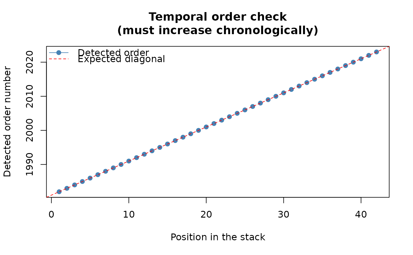#> Stack built: 42 layers, 146 x 338 cells.
#> >> [read_ordered_stack()] elapsed: 0.10 s

# Remove serial autocorrelation before testing for a trend -- only
# cells that actually show relevant autocorrelation are modified;
# the rest pass through unchanged.
result <- prewhiten(r, report = FALSE, verbose = FALSE)

# result$series is the prewhitened stack, same number of layers as the
# input -- feed this into trend_test()/slope_estimator()
# next, not the raw r.
terra::nlyr(result$series)
#> [1] 42
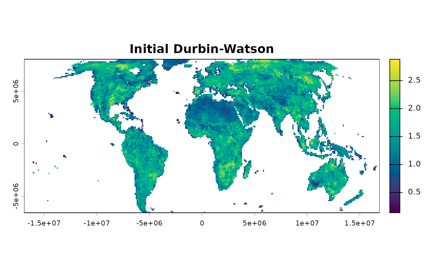
summary(result)
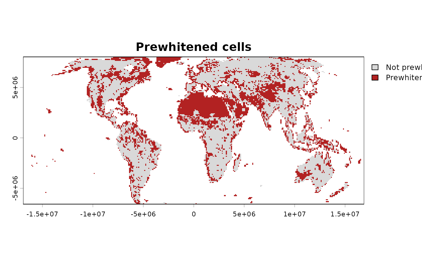
#> Valid cells: 15675
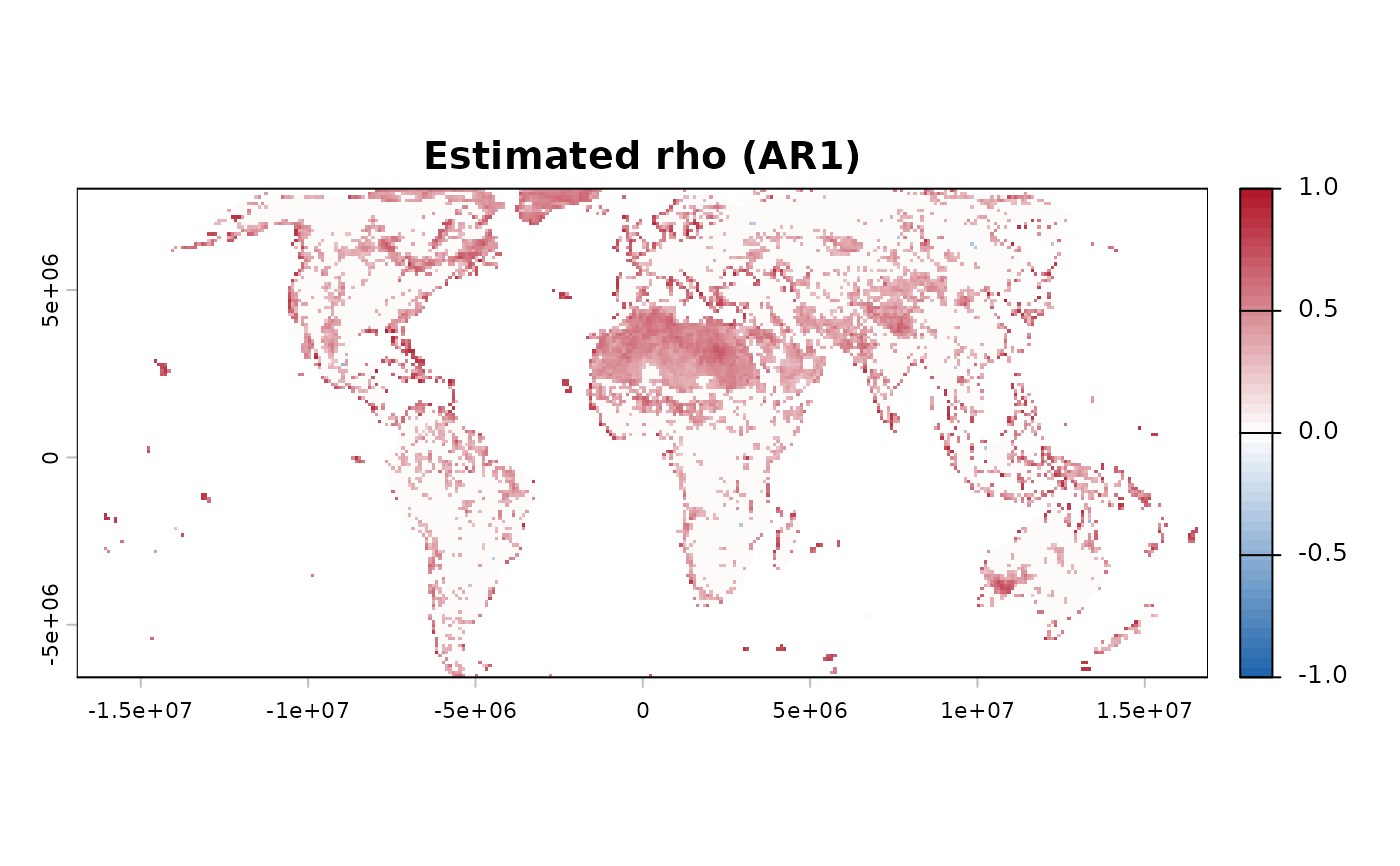
#> Prewhitened: 5987 (38.2%)
#> Mean rho among prewhitened cells: 0.4493
#> Median Durbin-Watson (all valid cells): 1.5306
plot(result)   # Rho map and the DW-before/after comparison, real data




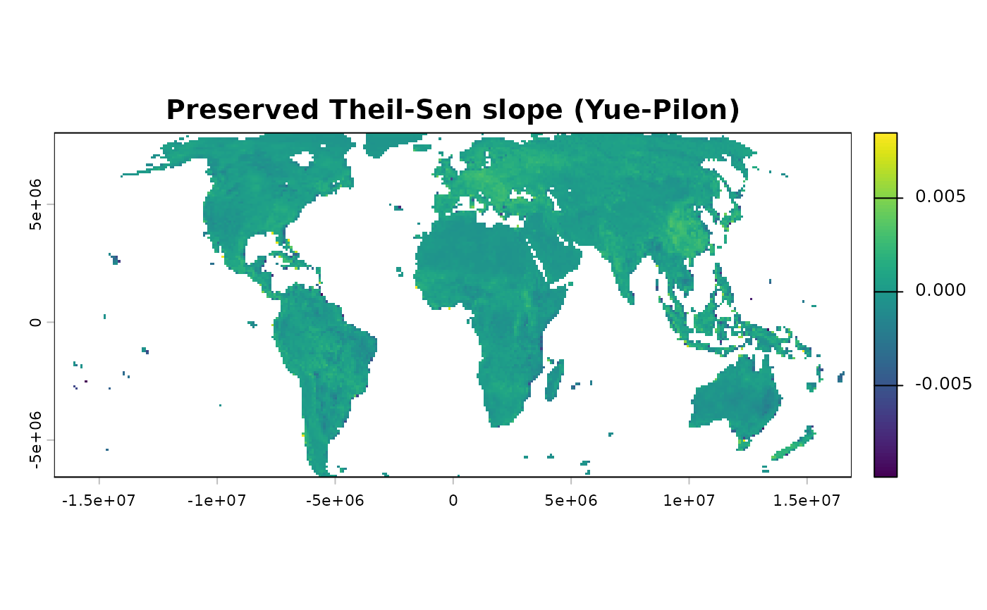
# Trend-free pre-whitening (Yue-Pilon): every valid cell is
# processed, its Theil-Sen trend preserved -- result_yp$series has
# one fewer layer than r (the classic transform loses the first
# time step to lag-1 differencing).
result_yp <- prewhiten(r, method = "TFPW_Y", report = FALSE,
                        verbose = FALSE)
terra::nlyr(result_yp$series)
#> [1] 41
terra::plot(result_yp$diagnostics$Beta_TheilSen,
            main = "Preserved Theil-Sen slope (Yue-Pilon)")

# }