Slope estimators for raster time series

Estimates the magnitude of a monotonic trend, independently of its statistical significance. trend_test() primarily tells you whether there is evidence of a trend and its direction; although its "OLS" branch necessarily returns a fitted coefficient, this function provides the dedicated and method-independent estimation of the rate of change, per cell, using one of three published estimators (see the method argument below).

Usage

slope_estimator(
  x,
  method = c("TS", "OLS", "RM"),
  t,
  max_pairs = 1e+05,
  seed = NULL,
  n_cores = 1,
  smooth_neighbourhood = FALSE,
  report = TRUE,
  verbose = TRUE,
  shared_cluster = NULL
)

Arguments

x

A terra::SpatRaster; each layer is one time step, in increasing chronological order.

method

Which slope estimator to use.

"TS" (default): the classic Theil-Sen estimator – the median of all pairwise slopes per cell, in the same units as x per unit of t. Robust (outlier-resistant) up to a ~29% breakdown point, at the cost of the performance profile described in "Computational considerations" below. This package's own default – see "Methodological details" below for why.

"OLS": ordinary least squares – the closed-form linear regression slope, cov(t, y) / var(t) per cell, computed directly with a single vectorised matrix operation (no pairwise sampling, no iteration – max_pairs, seed, and n_cores below are all ignored). Faster, and the more familiar choice to most users and to readers used to classical linear regression. Worth choosing over the default specifically when: speed matters more than robustness (very large rasters or very long series – see "Computational considerations" below); the residuals are genuinely expected to be close to normally distributed with no substantial outlier risk (in which case OLS is also the more statistically efficient of the two, with lower variance for the same data); or the result needs to be directly comparable to other analyses reported as classical linear-regression slopes, rather than a median-of-pairwise-slopes estimate.

"RM": Siegel's (1982) repeated median estimator – for each cell, the median slope from every observation to every other observation is computed first (one median per observation), then the median of those per-observation medians is taken as the final slope. Like "TS", median-based and highly robust – but with a 50% breakdown point rather than Theil-Sen's own ~29%, at a real computational cost: this is a naive O(n^2) port (see "Implementation notes" below), not the quasilinear-time algorithm the reference implementation this was ported from and verified against, robslopes::RepeatedMedian(), itself uses. Choose this over "TS" specifically when a dataset is suspected to have enough outliers or leverage points that Theil-Sen's own lower breakdown point might not fully resist them; max_pairs, seed and n_cores below are not used by this method (unlike "TS", it does not sample pairs, and is not currently parallelised).

t

Numeric vector of time points, one per layer. Defaults to 1:nlyr(x). Irregular spacing is supported, but values must be finite, unique and strictly increasing.

max_pairs

Integer or Inf. Only used when method = "TS". If the number of possible pairs (n*(n-1)/2) exceeds this, a random sample of max_pairs pairs is used per cell (see "Computational considerations" below). Default 100000; set to Inf for the exact computation regardless of series length.

seed

Integer or NULL. Only used when method = "TS" and subsampling actually happens (random seed for the pair sampling).

n_cores

Integer. Only used when method = "TS". Number of cores for the cell loop. 1 (default): sequential. > 1: uses a parallel::makeCluster() PSOCK cluster.

smooth_neighbourhood

Logical. Default FALSE – the estimated slope (whichever method was used) is left as computed, per cell independently. If TRUE, each cell's slope is replaced by the median of the already-estimated slopes in its queen 3x3 neighbourhood (itself and its 8 surrounding cells) – a queen-neighbourhood median filter applied to the per-cell slopes already computed, not a different way of estimating any individual cell's own slope. See the dedicated section below; read it before setting this to TRUE.

report

Logical. If TRUE (default), automatically print the summary (slope_summary()) and draw the map (slope_map()) once the slope finishes computing.

verbose

Logical. Print progress messages and elapsed time.

shared_cluster

Advanced; most users never need this directly. An already-running parallel::makeCluster() PSOCK cluster (e.g. from workflow_tst()'s own n_cores) to reuse instead of building a new one from n_cores above. When supplied, n_cores is ignored – the shared cluster's own size was already decided by whoever built it. NULL (default): builds and tears down its own cluster from n_cores, exactly as before this argument existed.

Value

Returns an object of class c("slope", "sptrends"): a list with

slope: A single-layer terra::SpatRaster, named "theilsen_slope", "ols_slope" or "rm_slope" depending on method (units: x per unit of t, e.g. per year if t is in years).
intercept: Only for method = "RM": a single-layer terra::SpatRaster (named "rm_intercept", NA for invalid cells), the repeated median estimator's own intercept – see "Implementation notes" below for how it is computed. Smoothed the same way slope itself is when smooth_neighbourhood = TRUE, for the same reason: a SpatRaster, matching slope's own representation, rather than a plain numeric vector.
method: Character: which method produced this result ("TS", "OLS" or "RM").
smoothed: Logical: whether post-estimation neighbourhood smoothing (smooth_neighbourhood = TRUE) was applied to slope after estimation, not whether smoothing was itself part of how slope was computed.

Use print()/summary()/plot() – see print.sptrends(), summary.sptrends(), and plot.sptrends().

Details

Function type: Companion function to trend_test() – one of the three quantities a standard trend analysis normally reports (alongside significance and multiple-testing correction), not a mere supporting utility, though not one of trend_test() or fdr_correction()'s own inferential building blocks either.

Typical use

raster time series
    |
slope_estimator()
    |
change per time unit (`result$slope`)

Run this beside trend_test() on the same analytical series: the slope measures magnitude, whereas the trend test assesses evidence. If the test uses a prewhitened series, choose deliberately whether the scientific estimand is the slope of that transformed series or of the original series.

Methodological details

Why estimate the slope separately from the trend test?

Statistical significance and effect size answer different questions. A statistically significant trend may be negligible in magnitude, whereas a large estimated slope may fail to reach significance when uncertainty is high. For this reason, sptrends separates trend testing (trend_test()) from slope estimation (this function), allowing each quantity to be interpreted independently – neither substitutes for the other.

Methods and method selection

Original publication: Theil (1950), later generalised by Sen (1968) into the median-of-pairwise-slopes form used here (linking it to Kendall's tau).
Main references: Theil (1950) and Sen (1968), the two papers this estimator is directly named after. Full citations in "References" below.
Typical applications: estimating the magnitude of a monotonic trend when the data may contain outliers or heavy-tailed noise – robust up to a ~29% breakdown point, unlike ordinary least squares.
Theil-Sen vs. OLS: both quantify a linear rate of change, but they define and estimate that rate differently, under different statistical assumptions – Theil-Sen makes no distributional assumption about the noise and tolerates a substantial fraction of outliers before breaking down; OLS is highly sensitive to influential observations and heavy-tailed errors. Normality is not required to calculate the OLS slope itself, although conventional small-sample inference for it (its own standard errors and significance test) relies on additional distributional assumptions the point estimate does not need. See the method argument below for when each is the more defensible choice.

Implementation notes (method = "RM" specifically)

"RM" implements Siegel's (1982) repeated median estimator using the upper-median convention robslopes::RepeatedMedian() itself uses: for a vector of length k, the upper median is sort(v)[floor((k + 2) / 2)]; this differs from stats::median(), which averages the two central observations when k is even.

This implementation computes the estimator directly in O(n^2) time. It therefore reproduces the estimator itself, but not the faster, quasilinear-time algorithm (Matousek, Mount and Netanyahu, 1998) robslopes uses internally in C++.

The intercept follows the "direct" (also called "separate") repeated-median convention, applying the same nested upper-median operation to the pairwise intercepts, rather than the simpler "hierarchical" convention (median(y - slope * t), using the already-computed overall slope) – both are legitimate conventions Siegel (1982) himself describes, but only the former matches robslopes::RepeatedMedian()'s own intercept output.

Statistical assumptions and interpretation

All methods require finite, unique and strictly increasing time values. Duplicates would produce undefined pairwise slopes for the robust estimators, while unordered values would no longer describe the chronological layer order; both are rejected before calculation. Valid cells must have a complete time series. Each estimator summarises change as one overall linear rate: "OLS" targets the least-squares slope, "TS" the median pairwise slope, and "RM" the repeated-median slope. The robust estimators do not require normally distributed errors; OLS can still be calculated without normality, but is more sensitive to outliers and influential observations.

Linear long-term change and seasonality

These estimators quantify an overall linear rate of change; they do not model seasonal cycles or nonlinear temporal structure. For strongly seasonal series, consider estimating the slope from anomalies (see compute_anomalies()) or using an appropriate seasonal model instead.

Computational considerations

Performance – read this before using long time series

The estimators have substantially different computational profiles. OLS is the fastest because it uses one vectorised closed-form calculation. Exact Theil-Sen is slower because it evaluates pairwise slopes, but it offers a strong practical balance between robustness, interpretation and computational cost and is therefore the recommended general-purpose estimator. The directly implemented repeated median is usually much slower than both because it calculates nested medians for every observation in every cell; reserve RM for cases in which its higher breakdown point is scientifically needed and its additional cost is acceptable.

The exact estimator needs every pairwise slope, n*(n-1)/2 of them per cell – unlike the Mann-Kendall S statistic, this cannot be accumulated as a running sum, so it does not benefit from the same O(n^2)-time-but-O(1)-memory trick. For a modest n (a few dozen time steps) this is fast. For long series (hundreds to thousands of steps – e.g. multi-decade monthly data) the number of pairs per cell can reach the hundreds of thousands, and computing an exact median that many times per cell, over every cell, gets slow. Two ways to cope:

n_cores > 1: splits cells across a parallel::makeCluster() PSOCK cluster (each cell's pairs still computed exactly).
max_pairs: if n*(n-1)/2 exceeds this, a random sample of max_pairs pairs is used per cell instead of the full set (a standard approximation for Theil-Sen on long series). Random pair sampling approximates the exact Theil-Sen slope; increasing max_pairs generally reduces Monte Carlo variability between runs and improves agreement with the exact estimate, though it is not guaranteed to be exactly unbiased in every finite sample. seed below controls the reproducibility of that approximation across runs. Set to Inf to force the exact computation regardless of n.

If speed genuinely matters more than robustness to outliers – very large rasters, very long series, and residuals not expected to be heavy-tailed or outlier-prone – method = "OLS" sidesteps this entire performance question: a single closed-form matrix operation, with no pairwise sampling and no per-cell iteration at all.

Optional queen-neighbourhood smoothing – read the caveats first

This is an optional visual/post-processing step, not part of the published Theil-Sen estimator itself.

What it does: smooth_neighbourhood = TRUE replaces each cell's slope with the median of its own slope and its 8 queen neighbours (a 3x3 focal median), computed after the per-cell Theil-Sen estimation above – it does not change how any individual cell's own slope is estimated.

What it does not inherit: this is not the same thing as trend_test()'s neighbourhood argument, and does not carry the same justification. CMK's neighbourhood-adjusted statistic follows a published, validated method (Neeti & Eastman, 2011) for the specific question "is there a trend", where borrowing spatial evidence for a yes/no decision is on solid ground. Smoothing the magnitude this way has no equivalent literature backing here – it assumes neighbouring cells share similar true slopes, which is not always true (e.g. a valley cell next to a sunlit slope can have a genuinely different real trend from its neighbours), and in that case this would blend two different real signals into one, less accurate, number for both.

When it might make sense: purely as a display/visual-smoothing aid for a map that will be read at a glance, where averaging out cell-to-cell estimation noise is more valuable than preserving every individual cell's own independent estimate – not as a way to "improve" the underlying statistic.

Warnings: off by default for the reasons above. If you use it, validate it first for your own data and resolution using sim_trend_stack() and compare_detections() against known ground truth, rather than judging it only by whether the smoothed map looks visually more coherent – a smoother-looking map is not the same as a more accurate one.

One thing this smoothing does not do: extend the footprint of "has data" beyond where data actually exists. A cell with no complete time series of its own (its own slope is NA) stays NA after smoothing, even if all 8 of its neighbours have valid slopes – terra::focal()'s own default behaviour would otherwise fill such a cell in from its neighbours, which would be presenting an estimate for a location that was never actually observed.

Limitations

These estimators describe one overall linear rate and do not identify breakpoints, nonlinear trajectories, or seasonal components. Cells with incomplete time series are returned as NA. Optional spatial smoothing changes the reported local magnitude and must not be interpreted as part of any of the three published estimators.

Quality assurance

Theil-Sen slopes are compared exactly with trend::sens.slope(), including tied data; OLS results are checked against stats::lm(); and repeated-median slopes and intercepts are checked against direct hand implementations. Automated tests also cover irregular time coordinates, missing and constant series, optional neighbourhood smoothing, raster return types, and sequential/parallel equivalence. See ?sptrends for the common release-check protocol.

References

method = "TS", original estimator:

Theil, H. (1950) A rank-invariant method of linear and polynomial regression analysis. Indagationes Mathematicae, 12, 85-91 (Part I; published in three parts). No DOI available (pre-DOI-era publication).

Generalisation into the median-of-pairwise-slopes estimator used by this function, linking it to Kendall's tau:

Sen, P.K. (1968) Estimates of the regression coefficient based on Kendall's tau. Journal of the American Statistical Association, 63, 1379-1389. doi:10.1080/01621459.1968.10480934

method = "OLS": the classical least-squares regression slope, independently attributed to both of the following (no single original paper; both pre-DOI-era):

Legendre, A.M. (1805) Nouvelles méthodes pour la détermination des orbites des comètes. Firmin Didot, Paris.
Gauss, C.F. (1809) Theoria motus corporum coelestium in sectionibus conicis solem ambientium. Perthes und Besser, Hamburg.

method = "RM", original estimator:

Siegel, A.F. (1982) Robust regression using repeated medians. Biometrika, 69(1), 242-244. doi:10.1093/biomet/69.1.242

The quasilinear-time algorithm the reference implementation this was ported from and verified against, robslopes::RepeatedMedian(), itself uses (not this package's own, deliberately simpler O(n^2) port – see "Implementation notes" above):

Matoušek, J., Mount, D.M. and Netanyahu, N.S. (1998) Efficient Randomized Algorithms for the Repeated Median Line Estimator. Algorithmica, 20(2), 136-150. doi:10.1007/PL00009190

Documents robslopes itself, including the exact formula and upper- median convention this port was verified against:

Raymaekers, J. (2023) robslopes: Efficient Computation of the (Repeated) Median Slope. The R Journal, 15(1), 249-260. doi:10.32614/RJ-2023-012

This function is used (not authored) by both of this package's own integrated workflows, workflow_tst() and workflow_rta(), and by the studies behind them:

Gutiérrez-Hernández, O. and García, L.V. (2025) Uncovering true significant trends in global greening. Remote Sensing Applications: Society and Environment, 37, 101377. doi:10.1016/j.rsase.2024.101377
Gutiérrez-Hernández, O. and García, L.V. (2024) Robust Trend Analysis in Environmental Remote Sensing: A Case Study of Cork Oak Forest Decline. Remote Sensing, 16(20), 3886. doi:10.3390/rs16203886

Examples

# \donttest{
# Annual mean NDVI from the bundled environmental dataset.
r <- read_ordered_stack(example_data("vhp_ndvi"))
#> Temporal order auto-detected with pattern '(19[0-9]{2}|20[0-9]{2})'.
#> Automatic mode: order detected from file names. For higher reliability -- especially if the series is not annual -- supplying 'files' explicitly (with 'time' or 'cycle_type') is recommended. See ?read_ordered_stack.
#> Temporal order verification (mandatory, cannot be skipped):
#>  stack_position detected_number                         file
#>               1            1982 VHP_SMN_annual_ndvi_1982.tif
#>               2            1983 VHP_SMN_annual_ndvi_1983.tif
#>               3            1984 VHP_SMN_annual_ndvi_1984.tif
#>               4            1985 VHP_SMN_annual_ndvi_1985.tif
#>               5            1986 VHP_SMN_annual_ndvi_1986.tif
#>               6            1987 VHP_SMN_annual_ndvi_1987.tif
#>               7            1988 VHP_SMN_annual_ndvi_1988.tif
#>               8            1989 VHP_SMN_annual_ndvi_1989.tif
#>               9            1990 VHP_SMN_annual_ndvi_1990.tif
#>              10            1991 VHP_SMN_annual_ndvi_1991.tif
#>              11            1992 VHP_SMN_annual_ndvi_1992.tif
#>              12            1993 VHP_SMN_annual_ndvi_1993.tif
#>              13            1994 VHP_SMN_annual_ndvi_1994.tif
#>              14            1995 VHP_SMN_annual_ndvi_1995.tif
#>              15            1996 VHP_SMN_annual_ndvi_1996.tif
#>              16            1997 VHP_SMN_annual_ndvi_1997.tif
#>              17            1998 VHP_SMN_annual_ndvi_1998.tif
#>              18            1999 VHP_SMN_annual_ndvi_1999.tif
#>              19            2000 VHP_SMN_annual_ndvi_2000.tif
#>              20            2001 VHP_SMN_annual_ndvi_2001.tif
#>              21            2002 VHP_SMN_annual_ndvi_2002.tif
#>              22            2003 VHP_SMN_annual_ndvi_2003.tif
#>              23            2004 VHP_SMN_annual_ndvi_2004.tif
#>              24            2005 VHP_SMN_annual_ndvi_2005.tif
#>              25            2006 VHP_SMN_annual_ndvi_2006.tif
#>              26            2007 VHP_SMN_annual_ndvi_2007.tif
#>              27            2008 VHP_SMN_annual_ndvi_2008.tif
#>              28            2009 VHP_SMN_annual_ndvi_2009.tif
#>              29            2010 VHP_SMN_annual_ndvi_2010.tif
#>              30            2011 VHP_SMN_annual_ndvi_2011.tif
#>              31            2012 VHP_SMN_annual_ndvi_2012.tif
#>              32            2013 VHP_SMN_annual_ndvi_2013.tif
#>              33            2014 VHP_SMN_annual_ndvi_2014.tif
#>              34            2015 VHP_SMN_annual_ndvi_2015.tif
#>              35            2016 VHP_SMN_annual_ndvi_2016.tif
#>              36            2017 VHP_SMN_annual_ndvi_2017.tif
#>              37            2018 VHP_SMN_annual_ndvi_2018.tif
#>              38            2019 VHP_SMN_annual_ndvi_2019.tif
#>              39            2020 VHP_SMN_annual_ndvi_2020.tif
#>              40            2021 VHP_SMN_annual_ndvi_2021.tif
#>              41            2022 VHP_SMN_annual_ndvi_2022.tif
#>              42            2023 VHP_SMN_annual_ndvi_2023.tif

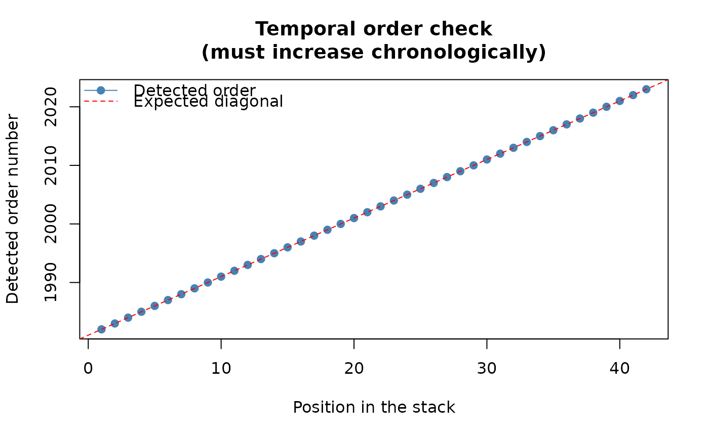#> Stack built: 42 layers, 146 x 338 cells.
#> >> [read_ordered_stack()] elapsed: 0.11 s

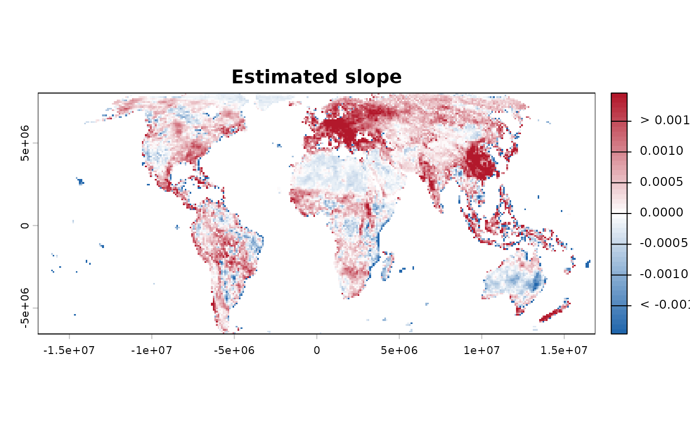
# The rate of change per cell, in NDVI units per year (the raster's
# own time unit) -- this is "how fast", not "is it significant" (that
# is what trend_test()/workflow_tst() answer instead).
result <- slope_estimator(r, verbose = FALSE, report = FALSE)

# A "slope" object: result$slope is the SpatRaster itself; plot() and
# summary() give the diverging map and the descriptive statistics
# without reconstructing either by hand.
plot(result)

summary(result)
#> Valid cells: 15675
#> Slope range: [-0.009883, 0.008481]
#> Median slope: 0.000279 | Mean slope: 0.0003253
#> Increasing: 10555 (67.3%) | Decreasing: 5101 (32.5%) | Flat: 19 (0.1%)

# Ordinary least squares: much faster (a single closed-form matrix
# operation, no pairwise sampling) -- see "Methodological details"
# for when this efficiency is, and is not, worth
# its own trade-offs relative to the two rank-based methods.
result_ols <- slope_estimator(r, method = "OLS", verbose = FALSE,
                               report = FALSE)
# }