
A quick, one-line-per-detail overview of any classed object this
package returns – workflow_tst(), workflow_rta(),
workflow_trends(),
trend_test(), slope_estimator(),
prewhiten(), and fdr_correction() all return an object
with "sptrends" as (one of) its classes, and print(),
summary.sptrends(), and plot.sptrends() all work the same way
regardless of which one you have – the specific one-line summary
shown depends on x's own class, listed below. This mirrors the
convention used throughout terra itself (a single print(),
whether x is a SpatRaster or a SpatVector): one predictable
entry point per generic, not a different function name to remember
for each result type. The API is organised around the object a
function returns, not around remembering which reporting function
goes with which: x <- workflow_tst(...), then print(x),
summary(x), plot(x), regardless of what x actually is.
Usage
# S3 method for class 'sptrends'
print(x, ...)
Arguments
- x
An object of class
"sptrends"(also one of"tst","rta","workflow_trends","trend_test","slope","prewhiten","fdr","spatial_autocorrelation","compare_detections","sptrends_simulation","sptrends_simulation_design", or"sptrends_benchmark"), fromworkflow_tst(),workflow_rta(),workflow_trends(),trend_test(),slope_estimator(),prewhiten(),fdr_correction(),spatial_autocorrelation(),compare_detections(),sim_trend_stack(),simulation_design(), orbenchmark_methods().- ...
Ignored.
Details
| Generic | Purpose |
print() | Quick overview |
summary() | Detailed textual report |
plot() | Visual exploration |
print() itself is intended for a quick inspection of an object at
the console; use summary.sptrends() for more detailed textual
reporting and plot.sptrends() for graphical exploration.
Function type: Reporting/derived function – presents an existing result and does not compute a new statistical estimate.
Methodological details
Published workflow: "tst".
Whether prewhitening ran, how many cells were tested, and how many
are significant after FDR correction (if run).
Published workflow: "rta".
The Theil-Sen slope range, the trend test's cell count, and how many
cells are significant after FDR-BH correction.
Configurable workflow: "workflow_trends".
The selected preprocessing, trend-test, slope and FDR stages,
including skipped optional stages and the qualified Moran assessment
when requested.
Trend estimation: "trend_test".
How many cells were tested, and how many are significant at the
conventional alpha=0.05 threshold, uncorrected.
Trend estimation: "slope".
How many cells have a valid slope, and its range.
Diagnostic: "prewhiten".
How many cells were prewhitened, out of how many valid cells.
Diagnostic: "fdr".
How many cells are significant under each method that was requested
(raw, BH, BKY, and BY, if it was explicitly requested – see
?fdr_correction's own method argument for why "BY" is opt-in,
not part of its own default).
Diagnostic: "spatial_autocorrelation".
Global results show the observed statistic (Moran's I or Getis-Ord
General G), its sign where applicable, and its permutation p-value.
Local results show the valid-cell count and the exploratory number of
cells below the raw alpha, followed by the route to
fdr_correction() for BH, BKY or BY.
Validation: "compare_detections".
The comparison table itself, printed as a plain data frame (this
class also inherits from "data.frame", so indexing, $, and so on
all work exactly as they would on any other one).
Simulation and benchmarking.
Simulation objects report their dimensions, dependence model and known
signal. Designs report scenario counts and varied factors. Benchmarks
report their stage, methods, scenarios, replicates and elapsed time.
See also
summary.sptrends() for detailed textual output and
plot.sptrends() for graphical exploration.
Examples
# \donttest{
# Annual mean NDVI from the bundled environmental dataset.
r <- read_ordered_stack(example_data("vhp_ndvi"))
#> Temporal order auto-detected with pattern '(19[0-9]{2}|20[0-9]{2})'.
#> Automatic mode: order detected from file names. For higher reliability -- especially if the series is not annual -- supplying 'files' explicitly (with 'time' or 'cycle_type') is recommended. See ?read_ordered_stack.
#> Temporal order verification (mandatory, cannot be skipped):
#> stack_position detected_number file
#> 1 1982 VHP_SMN_annual_ndvi_1982.tif
#> 2 1983 VHP_SMN_annual_ndvi_1983.tif
#> 3 1984 VHP_SMN_annual_ndvi_1984.tif
#> 4 1985 VHP_SMN_annual_ndvi_1985.tif
#> 5 1986 VHP_SMN_annual_ndvi_1986.tif
#> 6 1987 VHP_SMN_annual_ndvi_1987.tif
#> 7 1988 VHP_SMN_annual_ndvi_1988.tif
#> 8 1989 VHP_SMN_annual_ndvi_1989.tif
#> 9 1990 VHP_SMN_annual_ndvi_1990.tif
#> 10 1991 VHP_SMN_annual_ndvi_1991.tif
#> 11 1992 VHP_SMN_annual_ndvi_1992.tif
#> 12 1993 VHP_SMN_annual_ndvi_1993.tif
#> 13 1994 VHP_SMN_annual_ndvi_1994.tif
#> 14 1995 VHP_SMN_annual_ndvi_1995.tif
#> 15 1996 VHP_SMN_annual_ndvi_1996.tif
#> 16 1997 VHP_SMN_annual_ndvi_1997.tif
#> 17 1998 VHP_SMN_annual_ndvi_1998.tif
#> 18 1999 VHP_SMN_annual_ndvi_1999.tif
#> 19 2000 VHP_SMN_annual_ndvi_2000.tif
#> 20 2001 VHP_SMN_annual_ndvi_2001.tif
#> 21 2002 VHP_SMN_annual_ndvi_2002.tif
#> 22 2003 VHP_SMN_annual_ndvi_2003.tif
#> 23 2004 VHP_SMN_annual_ndvi_2004.tif
#> 24 2005 VHP_SMN_annual_ndvi_2005.tif
#> 25 2006 VHP_SMN_annual_ndvi_2006.tif
#> 26 2007 VHP_SMN_annual_ndvi_2007.tif
#> 27 2008 VHP_SMN_annual_ndvi_2008.tif
#> 28 2009 VHP_SMN_annual_ndvi_2009.tif
#> 29 2010 VHP_SMN_annual_ndvi_2010.tif
#> 30 2011 VHP_SMN_annual_ndvi_2011.tif
#> 31 2012 VHP_SMN_annual_ndvi_2012.tif
#> 32 2013 VHP_SMN_annual_ndvi_2013.tif
#> 33 2014 VHP_SMN_annual_ndvi_2014.tif
#> 34 2015 VHP_SMN_annual_ndvi_2015.tif
#> 35 2016 VHP_SMN_annual_ndvi_2016.tif
#> 36 2017 VHP_SMN_annual_ndvi_2017.tif
#> 37 2018 VHP_SMN_annual_ndvi_2018.tif
#> 38 2019 VHP_SMN_annual_ndvi_2019.tif
#> 39 2020 VHP_SMN_annual_ndvi_2020.tif
#> 40 2021 VHP_SMN_annual_ndvi_2021.tif
#> 41 2022 VHP_SMN_annual_ndvi_2022.tif
#> 42 2023 VHP_SMN_annual_ndvi_2023.tif
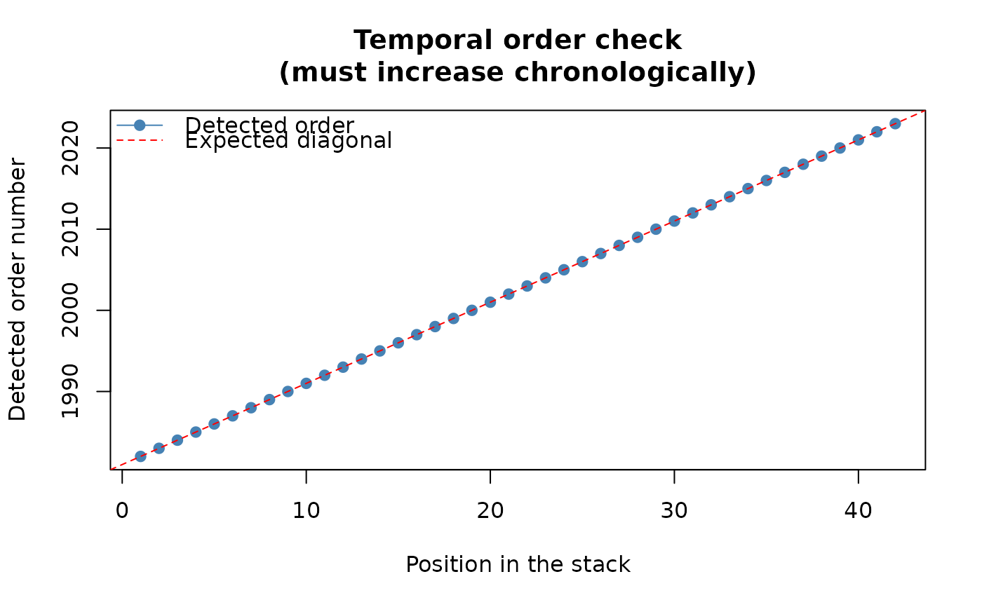 #> Stack built: 42 layers, 146 x 338 cells.
#> >> [read_ordered_stack()] elapsed: 0.10 s
result <- workflow_tst(r, report = FALSE, verbose = FALSE)
print(result) # dispatches to the "tst" case above
#> <True Significant Trends (TST) result>
#> Prewhitening: 5987 of 15675 cells modified (38.2%)
#> Trend test: 15675 cells (Sm statistic)
#> Theil-Sen slope: median 0.0002692 (range -0.01121 to 0.009657)
#> Significant after FDR-BKY: 7881 (50.3%)
#> Use summary() for details, plot() for a map.
# }
#> Stack built: 42 layers, 146 x 338 cells.
#> >> [read_ordered_stack()] elapsed: 0.10 s
result <- workflow_tst(r, report = FALSE, verbose = FALSE)
print(result) # dispatches to the "tst" case above
#> <True Significant Trends (TST) result>
#> Prewhitening: 5987 of 15675 cells modified (38.2%)
#> Trend test: 15675 cells (Sm statistic)
#> Theil-Sen slope: median 0.0002692 (range -0.01121 to 0.009657)
#> Significant after FDR-BKY: 7881 (50.3%)
#> Use summary() for details, plot() for a map.
# }