
The detailed textual report behind print()'s own one-line
overview – see print.sptrends() for the full class list and the
rationale for one shared entry point per generic. Each class here
calls its own underlying reporting function directly, listed below,
rather than duplicating what print() already shows.
Usage
# S3 method for class 'sptrends'
summary(object, ...)
Arguments
- object
An object of class
"sptrends"(also one of"tst","rta","workflow_trends","trend_test","slope","prewhiten","fdr","spatial_autocorrelation","compare_detections","sptrends_simulation","sptrends_simulation_design", or"sptrends_benchmark"), fromworkflow_tst(),workflow_rta(),workflow_trends(),trend_test(),slope_estimator(),prewhiten(),fdr_correction(),spatial_autocorrelation(),compare_detections(),sim_trend_stack(),simulation_design(), orbenchmark_methods().- ...
Passed on to the underlying reporting function (e.g.
path;alphafor"tst"/"rta"/"trend_test"objects).
Value
Invisibly, whatever the underlying reporting function itself returns – see each section below.
Details
Function type: Reporting/derived function – summarises an existing result and does not recompute its statistical analysis.
Methodological details
Published workflow: "tst".
The full detail behind the "tst" case of print.sptrends(): the
uncorrected trend summary table and, if FDR correction was run, the
FDR summary. Returns a list with trend and fdr (or NULL).
Published workflow: "rta".
The full detail behind the "rta" case of print.sptrends(): the
uncorrected trend summary table, the Theil-Sen slope summary, and the
FDR-BH summary. Returns a list with trend and fdr.
Configurable workflow: "workflow_trends".
The uncorrected trend table, optional slope summary and selected FDR
summary.
Trend estimation: "trend_test".
Cell counts and increase/decrease/no-change breakdown at multiple
alpha levels; calls trend_summary() internally.
Trend estimation: "slope".
Valid cells, range, median, mean, and the increasing/decreasing/flat
breakdown; calls slope_summary() internally.
Diagnostic: "prewhiten".
Valid cells, cells prewhitened, mean rho among them, and median
Durbin-Watson; calls prewhiten_summary() internally.
Diagnostic: "fdr".
Significant/not-significant counts and percentages for every method
requested; calls fdr_summary() internally.
Diagnostic: "spatial_autocorrelation".
Global results report the observed statistic, permutation distribution
and empirical summary statistics. Local results report the statistic
range, minimum permutation p-value and exploratory raw-significance
count.
Validation: "compare_detections".
Which method scores best on each numeric metric in the table – a
small table of its own, metric/best_method, not part of what
compare_detections() itself computes.
Simulation and benchmarking.
Simulation summaries quantify the true signal, true-null proportion and
slope range. Design summaries count levels per factor. Benchmark summaries
retain scenario factors and aggregate performance over independent Monte
Carlo replicates, including empirical FDR and FWER where available.
See also
print.sptrends() for a concise overview and
plot.sptrends() for graphical exploration.
Examples
# \donttest{
# Annual mean NDVI from the bundled environmental dataset.
r <- read_ordered_stack(example_data("vhp_ndvi"))
#> Temporal order auto-detected with pattern '(19[0-9]{2}|20[0-9]{2})'.
#> Automatic mode: order detected from file names. For higher reliability -- especially if the series is not annual -- supplying 'files' explicitly (with 'time' or 'cycle_type') is recommended. See ?read_ordered_stack.
#> Temporal order verification (mandatory, cannot be skipped):
#> stack_position detected_number file
#> 1 1982 VHP_SMN_annual_ndvi_1982.tif
#> 2 1983 VHP_SMN_annual_ndvi_1983.tif
#> 3 1984 VHP_SMN_annual_ndvi_1984.tif
#> 4 1985 VHP_SMN_annual_ndvi_1985.tif
#> 5 1986 VHP_SMN_annual_ndvi_1986.tif
#> 6 1987 VHP_SMN_annual_ndvi_1987.tif
#> 7 1988 VHP_SMN_annual_ndvi_1988.tif
#> 8 1989 VHP_SMN_annual_ndvi_1989.tif
#> 9 1990 VHP_SMN_annual_ndvi_1990.tif
#> 10 1991 VHP_SMN_annual_ndvi_1991.tif
#> 11 1992 VHP_SMN_annual_ndvi_1992.tif
#> 12 1993 VHP_SMN_annual_ndvi_1993.tif
#> 13 1994 VHP_SMN_annual_ndvi_1994.tif
#> 14 1995 VHP_SMN_annual_ndvi_1995.tif
#> 15 1996 VHP_SMN_annual_ndvi_1996.tif
#> 16 1997 VHP_SMN_annual_ndvi_1997.tif
#> 17 1998 VHP_SMN_annual_ndvi_1998.tif
#> 18 1999 VHP_SMN_annual_ndvi_1999.tif
#> 19 2000 VHP_SMN_annual_ndvi_2000.tif
#> 20 2001 VHP_SMN_annual_ndvi_2001.tif
#> 21 2002 VHP_SMN_annual_ndvi_2002.tif
#> 22 2003 VHP_SMN_annual_ndvi_2003.tif
#> 23 2004 VHP_SMN_annual_ndvi_2004.tif
#> 24 2005 VHP_SMN_annual_ndvi_2005.tif
#> 25 2006 VHP_SMN_annual_ndvi_2006.tif
#> 26 2007 VHP_SMN_annual_ndvi_2007.tif
#> 27 2008 VHP_SMN_annual_ndvi_2008.tif
#> 28 2009 VHP_SMN_annual_ndvi_2009.tif
#> 29 2010 VHP_SMN_annual_ndvi_2010.tif
#> 30 2011 VHP_SMN_annual_ndvi_2011.tif
#> 31 2012 VHP_SMN_annual_ndvi_2012.tif
#> 32 2013 VHP_SMN_annual_ndvi_2013.tif
#> 33 2014 VHP_SMN_annual_ndvi_2014.tif
#> 34 2015 VHP_SMN_annual_ndvi_2015.tif
#> 35 2016 VHP_SMN_annual_ndvi_2016.tif
#> 36 2017 VHP_SMN_annual_ndvi_2017.tif
#> 37 2018 VHP_SMN_annual_ndvi_2018.tif
#> 38 2019 VHP_SMN_annual_ndvi_2019.tif
#> 39 2020 VHP_SMN_annual_ndvi_2020.tif
#> 40 2021 VHP_SMN_annual_ndvi_2021.tif
#> 41 2022 VHP_SMN_annual_ndvi_2022.tif
#> 42 2023 VHP_SMN_annual_ndvi_2023.tif
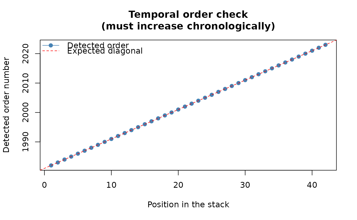 #> Stack built: 42 layers, 146 x 338 cells.
#> >> [read_ordered_stack()] elapsed: 0.12 s
result <- workflow_tst(r, report = FALSE, verbose = FALSE)
summary(result) # dispatches to the "tst" case above
#> === FDR correction (the actual TST result) ===
#> Valid cells (m): 15675 | target q: 0.05
#> BKY -- pi0_hat: 0.574992 | m0_hat: 9013.0 | r1 (stage 1): 6662
#>
#> === Theil-Sen slope ===
#> Min. 1st Qu. Median Mean 3rd Qu. Max. NAs
#> -0.0112134 -0.0001525 0.0002692 0.0003020 0.0007519 0.0096566 33673
#>
#> === Trend test, uncorrected (diagnostic only -- not the TST result; see FDR correction above) ===
#> alpha n_significant n_not_significant pct_significant n_valid
#> 1 0.05 8091 7584 51.62 15675
# }
#> Stack built: 42 layers, 146 x 338 cells.
#> >> [read_ordered_stack()] elapsed: 0.12 s
result <- workflow_tst(r, report = FALSE, verbose = FALSE)
summary(result) # dispatches to the "tst" case above
#> === FDR correction (the actual TST result) ===
#> Valid cells (m): 15675 | target q: 0.05
#> BKY -- pi0_hat: 0.574992 | m0_hat: 9013.0 | r1 (stage 1): 6662
#>
#> === Theil-Sen slope ===
#> Min. 1st Qu. Median Mean 3rd Qu. Max. NAs
#> -0.0112134 -0.0001525 0.0002692 0.0003020 0.0007519 0.0096566 33673
#>
#> === Trend test, uncorrected (diagnostic only -- not the TST result; see FDR correction above) ===
#> alpha n_significant n_not_significant pct_significant n_valid
#> 1 0.05 8091 7584 51.62 15675
# }