
Builds the sparse adjacency matrix (W[i,j] = 1 if j is a queen
neighbour of i and both have complete data) and the valid-neighbour
count per cell. Kept separate from trend_test() so it can
be reused without recomputation when the test is called repeatedly on
the same raster geometry (e.g. inside a permutation loop).
Arguments
- x
A
terra::SpatRasterdefining the geometry.- ok
Logical vector, length
ncell(x):TRUEwhere the cell has a complete time series.- connectivity
"queen"(default) or"rook".- window_size
Odd integer greater than or equal to
3. Width and height, in raster cells, of the moving neighbourhood. The default3Lreproduces the CMK region described by Neeti and Eastman (2011), as implemented in TerrSet's Kendall module.
Value
A list with W (sparse adjacency Matrix), nb_count
(numeric vector, valid-neighbour count per cell), and an internal
geometry/valid-cell signature used to reject unsafe reuse.
Details
Function type: Support function – computes something real,
but is not one of the
core building blocks of TST or RTA (used internally by, or as a
standalone diagnostic alongside, the core functions). Called
internally by trend_test() whenever precomputed_neighbourhood
isn't supplied; exported directly for the repeated-call optimisation
described above, since there is no single-object S3 method this
folds into (it takes a raw geometry and a logical vector, not a
classed result).
References
Neeti, N. and Eastman, J.R. (2011) A Contextual Mann-Kendall Approach for the Assessment of Trend Significance in Image Time Series. Transactions in GIS, 15(5), 599-611. doi:10.1111/j.1467-9671.2011.01280.x
See also
Other Contextual Mann-Kendall functions:
trend_histograms(),
trend_maps(),
trend_summary()
Examples
r <- read_ordered_stack(example_data("vhp_ndvi"))
#> Temporal order auto-detected with pattern '(19[0-9]{2}|20[0-9]{2})'.
#> Automatic mode: order detected from file names. For higher reliability -- especially if the series is not annual -- supplying 'files' explicitly (with 'time' or 'cycle_type') is recommended. See ?read_ordered_stack.
#> Temporal order verification (mandatory, cannot be skipped):
#> stack_position detected_number file
#> 1 1982 VHP_SMN_annual_ndvi_1982.tif
#> 2 1983 VHP_SMN_annual_ndvi_1983.tif
#> 3 1984 VHP_SMN_annual_ndvi_1984.tif
#> 4 1985 VHP_SMN_annual_ndvi_1985.tif
#> 5 1986 VHP_SMN_annual_ndvi_1986.tif
#> 6 1987 VHP_SMN_annual_ndvi_1987.tif
#> 7 1988 VHP_SMN_annual_ndvi_1988.tif
#> 8 1989 VHP_SMN_annual_ndvi_1989.tif
#> 9 1990 VHP_SMN_annual_ndvi_1990.tif
#> 10 1991 VHP_SMN_annual_ndvi_1991.tif
#> 11 1992 VHP_SMN_annual_ndvi_1992.tif
#> 12 1993 VHP_SMN_annual_ndvi_1993.tif
#> 13 1994 VHP_SMN_annual_ndvi_1994.tif
#> 14 1995 VHP_SMN_annual_ndvi_1995.tif
#> 15 1996 VHP_SMN_annual_ndvi_1996.tif
#> 16 1997 VHP_SMN_annual_ndvi_1997.tif
#> 17 1998 VHP_SMN_annual_ndvi_1998.tif
#> 18 1999 VHP_SMN_annual_ndvi_1999.tif
#> 19 2000 VHP_SMN_annual_ndvi_2000.tif
#> 20 2001 VHP_SMN_annual_ndvi_2001.tif
#> 21 2002 VHP_SMN_annual_ndvi_2002.tif
#> 22 2003 VHP_SMN_annual_ndvi_2003.tif
#> 23 2004 VHP_SMN_annual_ndvi_2004.tif
#> 24 2005 VHP_SMN_annual_ndvi_2005.tif
#> 25 2006 VHP_SMN_annual_ndvi_2006.tif
#> 26 2007 VHP_SMN_annual_ndvi_2007.tif
#> 27 2008 VHP_SMN_annual_ndvi_2008.tif
#> 28 2009 VHP_SMN_annual_ndvi_2009.tif
#> 29 2010 VHP_SMN_annual_ndvi_2010.tif
#> 30 2011 VHP_SMN_annual_ndvi_2011.tif
#> 31 2012 VHP_SMN_annual_ndvi_2012.tif
#> 32 2013 VHP_SMN_annual_ndvi_2013.tif
#> 33 2014 VHP_SMN_annual_ndvi_2014.tif
#> 34 2015 VHP_SMN_annual_ndvi_2015.tif
#> 35 2016 VHP_SMN_annual_ndvi_2016.tif
#> 36 2017 VHP_SMN_annual_ndvi_2017.tif
#> 37 2018 VHP_SMN_annual_ndvi_2018.tif
#> 38 2019 VHP_SMN_annual_ndvi_2019.tif
#> 39 2020 VHP_SMN_annual_ndvi_2020.tif
#> 40 2021 VHP_SMN_annual_ndvi_2021.tif
#> 41 2022 VHP_SMN_annual_ndvi_2022.tif
#> 42 2023 VHP_SMN_annual_ndvi_2023.tif
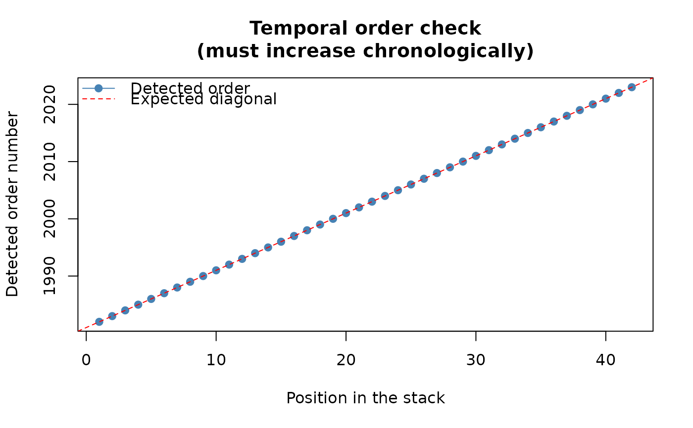 #> Stack built: 42 layers, 146 x 338 cells.
#> >> [read_ordered_stack()] elapsed: 0.12 s
# A matrix with one row per cell and one column per time step, and a
# logical vector marking which cells have a complete (no-NA) series --
# both are what trend_test() needs internally.
X <- terra::values(r, mat = TRUE)
ok <- stats::complete.cases(X)
# Precomputes the spatial adjacency (queen/rook neighbourhood) once,
# so it can be reused across repeated calls instead of recomputed
# every time -- see the precomputed_neighbourhood argument of
# trend_test().
nb <- prepare_cmk_neighbourhood(r, ok, window_size = 3)
names(nb)
#> [1] "W" "nb_count" "signature"
#> Stack built: 42 layers, 146 x 338 cells.
#> >> [read_ordered_stack()] elapsed: 0.12 s
# A matrix with one row per cell and one column per time step, and a
# logical vector marking which cells have a complete (no-NA) series --
# both are what trend_test() needs internally.
X <- terra::values(r, mat = TRUE)
ok <- stats::complete.cases(X)
# Precomputes the spatial adjacency (queen/rook neighbourhood) once,
# so it can be reused across repeated calls instead of recomputed
# every time -- see the precomputed_neighbourhood argument of
# trend_test().
nb <- prepare_cmk_neighbourhood(r, ok, window_size = 3)
names(nb)
#> [1] "W" "nb_count" "signature"