Function type: Reporting/derived function – summarises or
plots the output of
another function; it does not compute any new statistic. Not
exported – called internally by report = TRUE, and reachable
from outside the package via plot().
Usage
trend_maps(
  trend,
  alpha = 0.05,
  panels = c("statistic", "pvalue", "significance", "direction"),
  path = NULL
)
Arguments
- trend
The
$statsfield oftrend_test()'s output.- alpha
Numeric. Significance threshold used for the significance and direction-of-change maps. Uncorrected for multiple testing across cells – these maps are diagnostic, not a final significance result; run
fdr_correction()ontrend$p(and considerdirection_map()instead) before reporting which cells are significant.- panels
Character vector: which of the 4 available maps to draw, any subset of
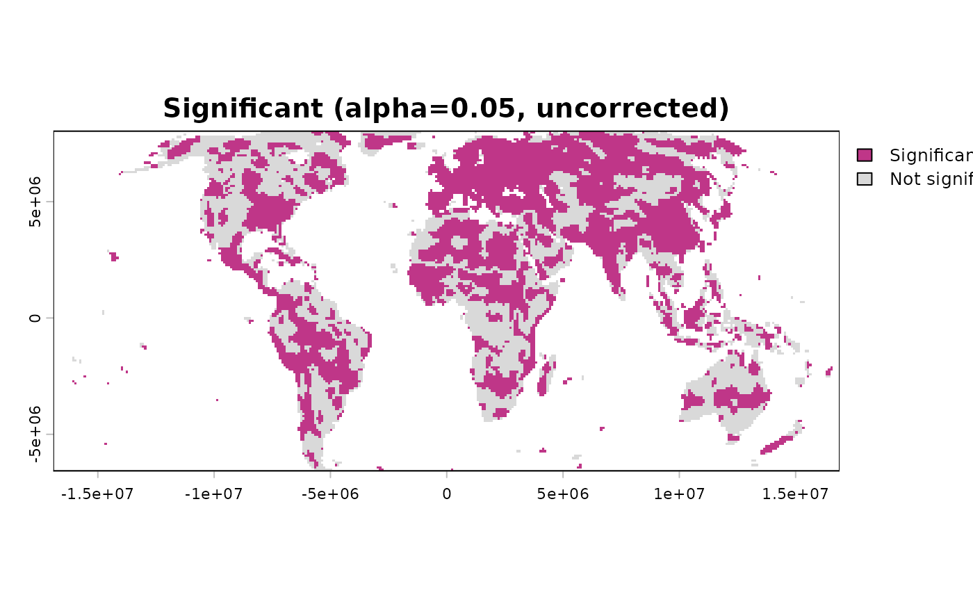
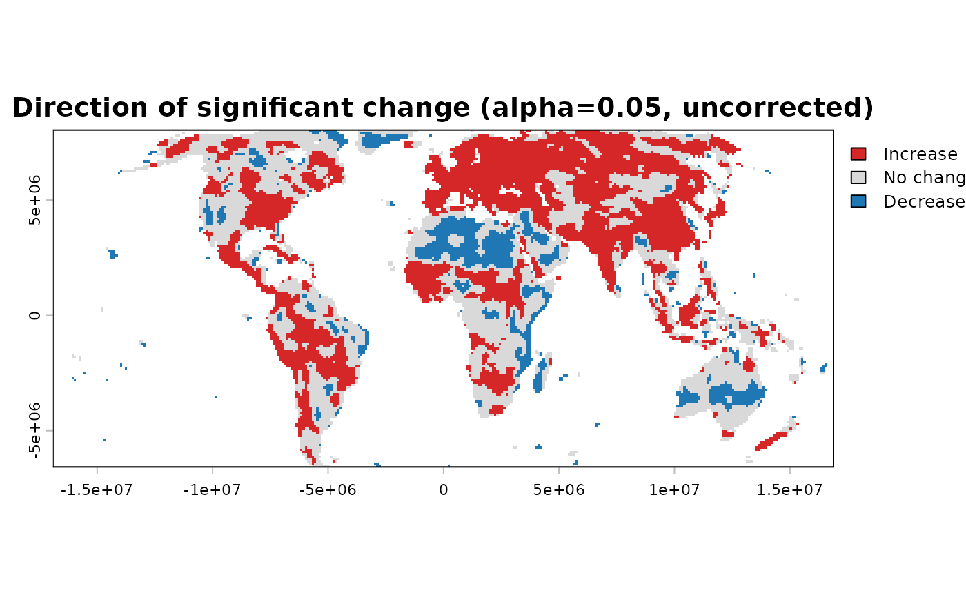
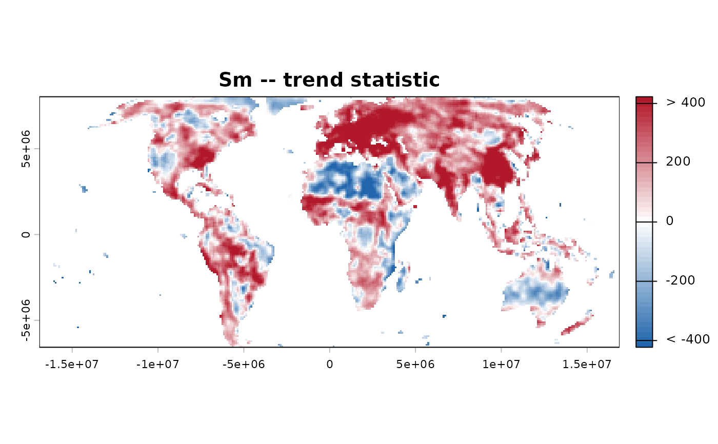
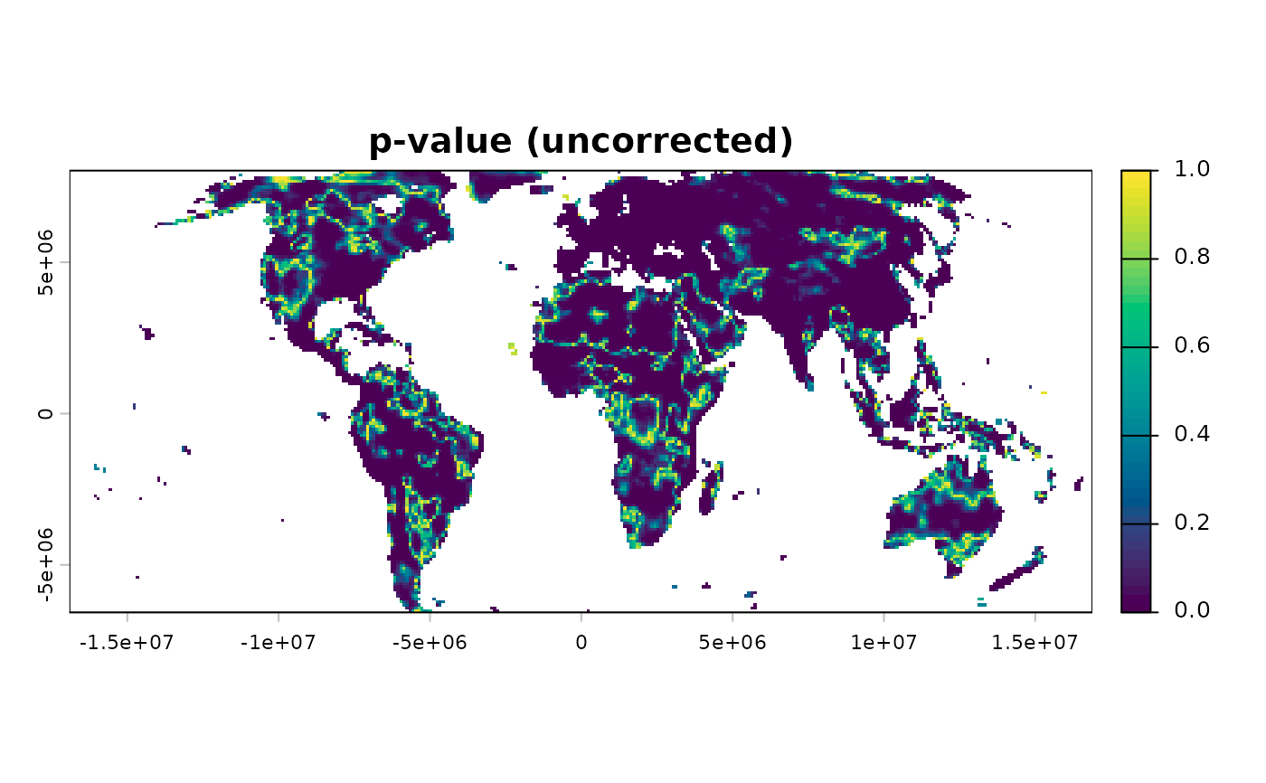
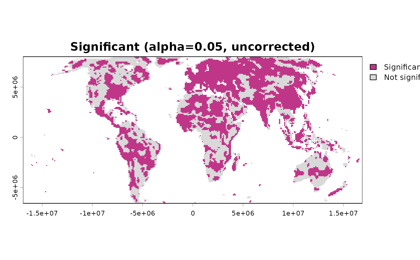
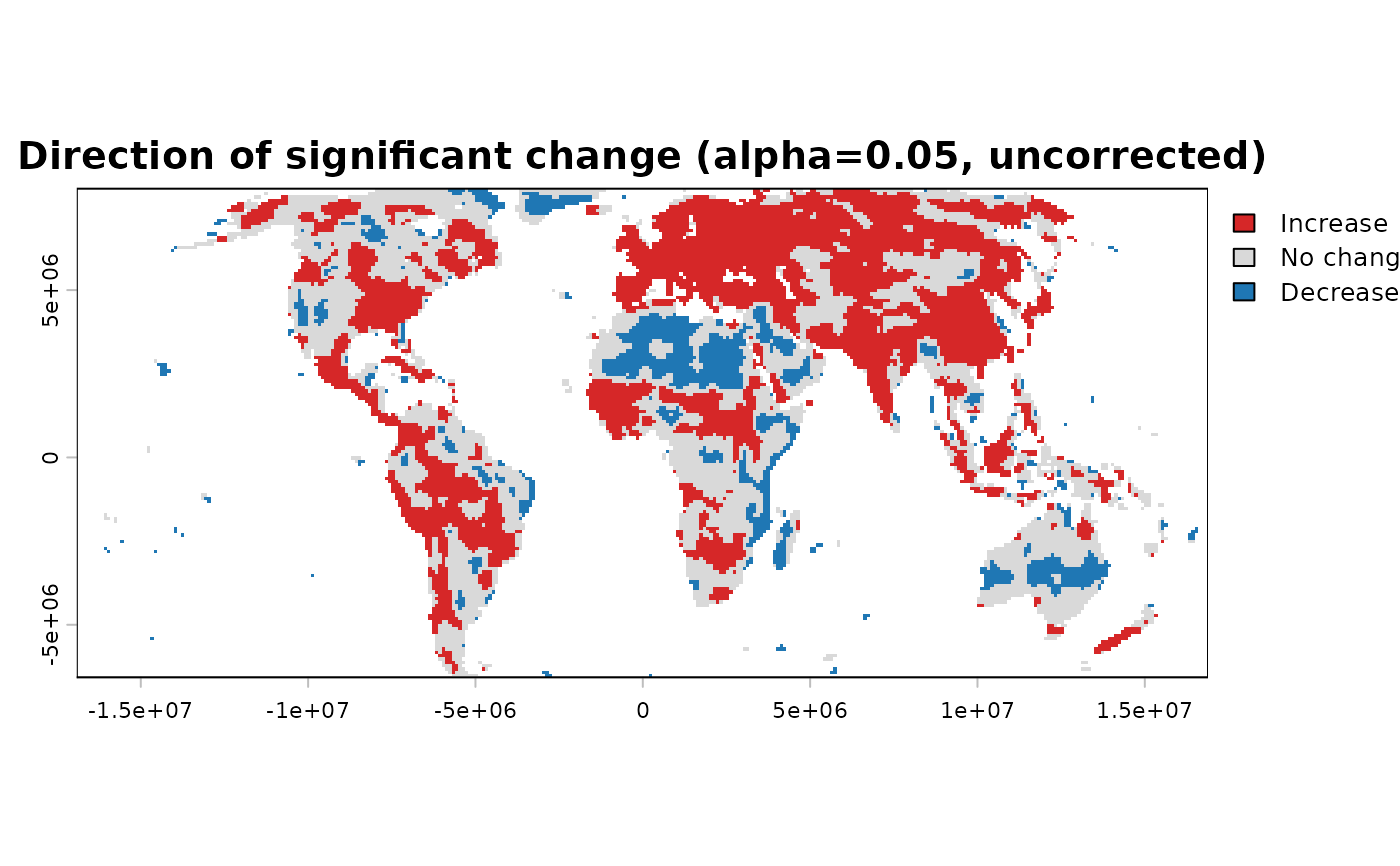
c("statistic", "pvalue", "significance", "direction")(default: all four, in that order)."statistic": the rawSm/Strend statistic (diverging)."pvalue": the uncorrected p-value (sequential)."significance": which cells crossalpha(binary)."direction": increase/decrease/no-change among the significant cells. Reachable viaplot(x, panels = ...)on atrend_test()result, which forwards this argument through.- path
Character or
NULL. If supplied, PNGs are written using this as a filename prefix.
Value
Invisibly, a list with significant and classes (both
SpatRaster, NULL if "significance"/"direction" respectively
was not in panels).
References
Neeti, N. and Eastman, J.R. (2011) A Contextual Mann-Kendall Approach for the Assessment of Trend Significance in Image Time Series. Transactions in GIS, 15(5), 599-611. doi:10.1111/j.1467-9671.2011.01280.x
See also
Other Contextual Mann-Kendall functions:
prepare_cmk_neighbourhood(),
trend_histograms(),
trend_summary()
Examples
r <- read_ordered_stack(example_data("vhp_ndvi"))
#> Temporal order auto-detected with pattern '(19[0-9]{2}|20[0-9]{2})'.
#> Automatic mode: order detected from file names. For higher reliability -- especially if the series is not annual -- supplying 'files' explicitly (with 'time' or 'cycle_type') is recommended. See ?read_ordered_stack.
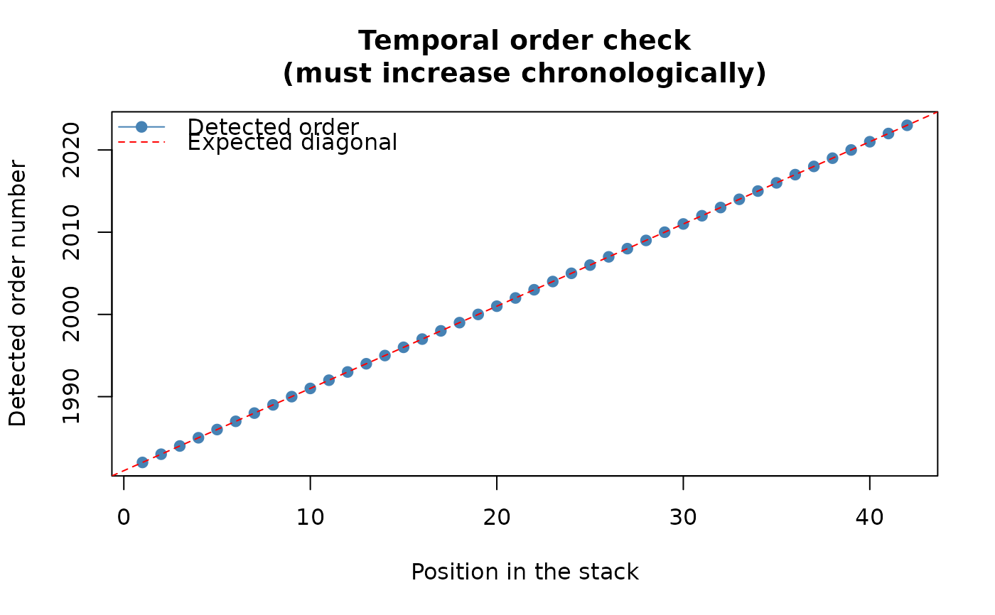
#> Temporal order verification (mandatory, cannot be skipped):
#> stack_position detected_number file
#> 1 1982 VHP_SMN_annual_ndvi_1982.tif
#> 2 1983 VHP_SMN_annual_ndvi_1983.tif
#> 3 1984 VHP_SMN_annual_ndvi_1984.tif
#> 4 1985 VHP_SMN_annual_ndvi_1985.tif
#> 5 1986 VHP_SMN_annual_ndvi_1986.tif
#> 6 1987 VHP_SMN_annual_ndvi_1987.tif
#> 7 1988 VHP_SMN_annual_ndvi_1988.tif
#> 8 1989 VHP_SMN_annual_ndvi_1989.tif
#> 9 1990 VHP_SMN_annual_ndvi_1990.tif
#> 10 1991 VHP_SMN_annual_ndvi_1991.tif
#> 11 1992 VHP_SMN_annual_ndvi_1992.tif
#> 12 1993 VHP_SMN_annual_ndvi_1993.tif
#> 13 1994 VHP_SMN_annual_ndvi_1994.tif
#> 14 1995 VHP_SMN_annual_ndvi_1995.tif
#> 15 1996 VHP_SMN_annual_ndvi_1996.tif
#> 16 1997 VHP_SMN_annual_ndvi_1997.tif
#> 17 1998 VHP_SMN_annual_ndvi_1998.tif
#> 18 1999 VHP_SMN_annual_ndvi_1999.tif
#> 19 2000 VHP_SMN_annual_ndvi_2000.tif
#> 20 2001 VHP_SMN_annual_ndvi_2001.tif
#> 21 2002 VHP_SMN_annual_ndvi_2002.tif
#> 22 2003 VHP_SMN_annual_ndvi_2003.tif
#> 23 2004 VHP_SMN_annual_ndvi_2004.tif
#> 24 2005 VHP_SMN_annual_ndvi_2005.tif
#> 25 2006 VHP_SMN_annual_ndvi_2006.tif
#> 26 2007 VHP_SMN_annual_ndvi_2007.tif
#> 27 2008 VHP_SMN_annual_ndvi_2008.tif
#> 28 2009 VHP_SMN_annual_ndvi_2009.tif
#> 29 2010 VHP_SMN_annual_ndvi_2010.tif
#> 30 2011 VHP_SMN_annual_ndvi_2011.tif
#> 31 2012 VHP_SMN_annual_ndvi_2012.tif
#> 32 2013 VHP_SMN_annual_ndvi_2013.tif
#> 33 2014 VHP_SMN_annual_ndvi_2014.tif
#> 34 2015 VHP_SMN_annual_ndvi_2015.tif
#> 35 2016 VHP_SMN_annual_ndvi_2016.tif
#> 36 2017 VHP_SMN_annual_ndvi_2017.tif
#> 37 2018 VHP_SMN_annual_ndvi_2018.tif
#> 38 2019 VHP_SMN_annual_ndvi_2019.tif
#> 39 2020 VHP_SMN_annual_ndvi_2020.tif
#> 40 2021 VHP_SMN_annual_ndvi_2021.tif
#> 41 2022 VHP_SMN_annual_ndvi_2022.tif
#> 42 2023 VHP_SMN_annual_ndvi_2023.tif
 #> Stack built: 42 layers, 146 x 338 cells.
#> >> [read_ordered_stack()] elapsed: 0.10 s
trend <- trend_test(r, report = FALSE, verbose = FALSE)
# All four maps: the trend statistic, the (uncorrected) p-value, which
# cells cross alpha = 0.05, and the direction of change among those.
plot(trend)
#> Stack built: 42 layers, 146 x 338 cells.
#> >> [read_ordered_stack()] elapsed: 0.10 s
trend <- trend_test(r, report = FALSE, verbose = FALSE)
# All four maps: the trend statistic, the (uncorrected) p-value, which
# cells cross alpha = 0.05, and the direction of change among those.
plot(trend)
 # Just the two most commonly wanted together -- raw/binary
# significance and direction -- skipping the statistic and p-value
# panels, whose raw scale is harder to read at a glance than a
# simple yes/no or increase/decrease map.
plot(trend, panels = c("significance", "direction"))
# Just the two most commonly wanted together -- raw/binary
# significance and direction -- skipping the statistic and p-value
# panels, whose raw scale is harder to read at a glance than a
# simple yes/no or increase/decrease map.
plot(trend, panels = c("significance", "direction"))