
Combines the sign of the trend statistic (Sm/S) with a chosen
FDR-corrected (or raw) rejection vector to classify each cell as an
increase, a decrease, or a non-significant result – a binarised map
for reporting after multiple-comparison correction, as
opposed to trend_maps(), which uses the uncorrected p-value.
Usage
direction_map(
  trend,
  fdr_result,
  slope = NULL,
  method = c("BH", "BKY", "BY", "raw"),
  verbose = TRUE
)
Arguments
- trend
The
$statsfield oftrend_test()'s output.- fdr_result
Output of
fdr_correction(), run ontrend$stats$p.- slope
Optional single-layer
SpatRaster(e.g.slope_estimator()'s own$slope) whose sign determines direction instead of the trend test's own statistic.NULL(default): usetrend's ownSm/S/beta, as before. Direction from the slope and direction from the trend statistic usually agree but are not guaranteed to: a cell with a near-flat slope of its own can still inherit its neighbours' sign inSmunder CMK's neighbourhood averaging. The significance mask (which cells are shown as increasing/decreasing at all, fromfdr_result) is identical either way – only the source of the sign for already-significant cells changes.- method
"BH"(default),"BKY","BY", or"raw"(uncorrected, included for comparison) – which rejection vector infdr_resultto use as the significance mask.- verbose
Logical. Print a one-line count summary.
Value
A single-layer terra::SpatRaster, values -1 (significant
decrease), 0 (not significant), 1 (significant increase), named
"binarised_trend_map".
Details
Function type: Support function – computes something real
(a genuinely new
raster, combining trend direction with significance), but is not one
of the core building blocks of TST or RTA itself; it is a
post-processing step that consumes the output of two of them
(trend_test() and fdr_correction()) together. Not exported –
the binarised trend direction is the same underlying
computation as the uncorrected direction already reachable via
plot(x, which = "trend"), just with a significance filter applied
on top; reachable directly via plot(x, which = "direction") for
workflow_tst()/workflow_rta() results, or with ::: for
programmatic use.
References
This combination of FDR-corrected significance with trend direction is this package's own contribution, not from an external method paper; cited here as the source of the overall TST workflow it belongs to:
Gutiérrez-Hernández, O. and García, L.V. (2025) Uncovering true significant trends in global greening. Remote Sensing Applications: Society and Environment, 37, 101377. doi:10.1016/j.rsase.2024.101377
Underlying theoretical justification for the FDR-BH assumption this significance is based on:
Benjamini, Y., & Yekutieli, D. (2001) The control of the false discovery rate in multiple testing under dependency. Annals of Statistics, 29(4), 1165-1188. doi:10.1214/aos/1013699998
Examples
# \donttest{
r <- read_ordered_stack(example_data("vhp_ndvi"))
#> Temporal order auto-detected with pattern '(19[0-9]{2}|20[0-9]{2})'.
#> Automatic mode: order detected from file names. For higher reliability -- especially if the series is not annual -- supplying 'files' explicitly (with 'time' or 'cycle_type') is recommended. See ?read_ordered_stack.
#> Temporal order verification (mandatory, cannot be skipped):
#> stack_position detected_number file
#> 1 1982 VHP_SMN_annual_ndvi_1982.tif
#> 2 1983 VHP_SMN_annual_ndvi_1983.tif
#> 3 1984 VHP_SMN_annual_ndvi_1984.tif
#> 4 1985 VHP_SMN_annual_ndvi_1985.tif
#> 5 1986 VHP_SMN_annual_ndvi_1986.tif
#> 6 1987 VHP_SMN_annual_ndvi_1987.tif
#> 7 1988 VHP_SMN_annual_ndvi_1988.tif
#> 8 1989 VHP_SMN_annual_ndvi_1989.tif
#> 9 1990 VHP_SMN_annual_ndvi_1990.tif
#> 10 1991 VHP_SMN_annual_ndvi_1991.tif
#> 11 1992 VHP_SMN_annual_ndvi_1992.tif
#> 12 1993 VHP_SMN_annual_ndvi_1993.tif
#> 13 1994 VHP_SMN_annual_ndvi_1994.tif
#> 14 1995 VHP_SMN_annual_ndvi_1995.tif
#> 15 1996 VHP_SMN_annual_ndvi_1996.tif
#> 16 1997 VHP_SMN_annual_ndvi_1997.tif
#> 17 1998 VHP_SMN_annual_ndvi_1998.tif
#> 18 1999 VHP_SMN_annual_ndvi_1999.tif
#> 19 2000 VHP_SMN_annual_ndvi_2000.tif
#> 20 2001 VHP_SMN_annual_ndvi_2001.tif
#> 21 2002 VHP_SMN_annual_ndvi_2002.tif
#> 22 2003 VHP_SMN_annual_ndvi_2003.tif
#> 23 2004 VHP_SMN_annual_ndvi_2004.tif
#> 24 2005 VHP_SMN_annual_ndvi_2005.tif
#> 25 2006 VHP_SMN_annual_ndvi_2006.tif
#> 26 2007 VHP_SMN_annual_ndvi_2007.tif
#> 27 2008 VHP_SMN_annual_ndvi_2008.tif
#> 28 2009 VHP_SMN_annual_ndvi_2009.tif
#> 29 2010 VHP_SMN_annual_ndvi_2010.tif
#> 30 2011 VHP_SMN_annual_ndvi_2011.tif
#> 31 2012 VHP_SMN_annual_ndvi_2012.tif
#> 32 2013 VHP_SMN_annual_ndvi_2013.tif
#> 33 2014 VHP_SMN_annual_ndvi_2014.tif
#> 34 2015 VHP_SMN_annual_ndvi_2015.tif
#> 35 2016 VHP_SMN_annual_ndvi_2016.tif
#> 36 2017 VHP_SMN_annual_ndvi_2017.tif
#> 37 2018 VHP_SMN_annual_ndvi_2018.tif
#> 38 2019 VHP_SMN_annual_ndvi_2019.tif
#> 39 2020 VHP_SMN_annual_ndvi_2020.tif
#> 40 2021 VHP_SMN_annual_ndvi_2021.tif
#> 41 2022 VHP_SMN_annual_ndvi_2022.tif
#> 42 2023 VHP_SMN_annual_ndvi_2023.tif
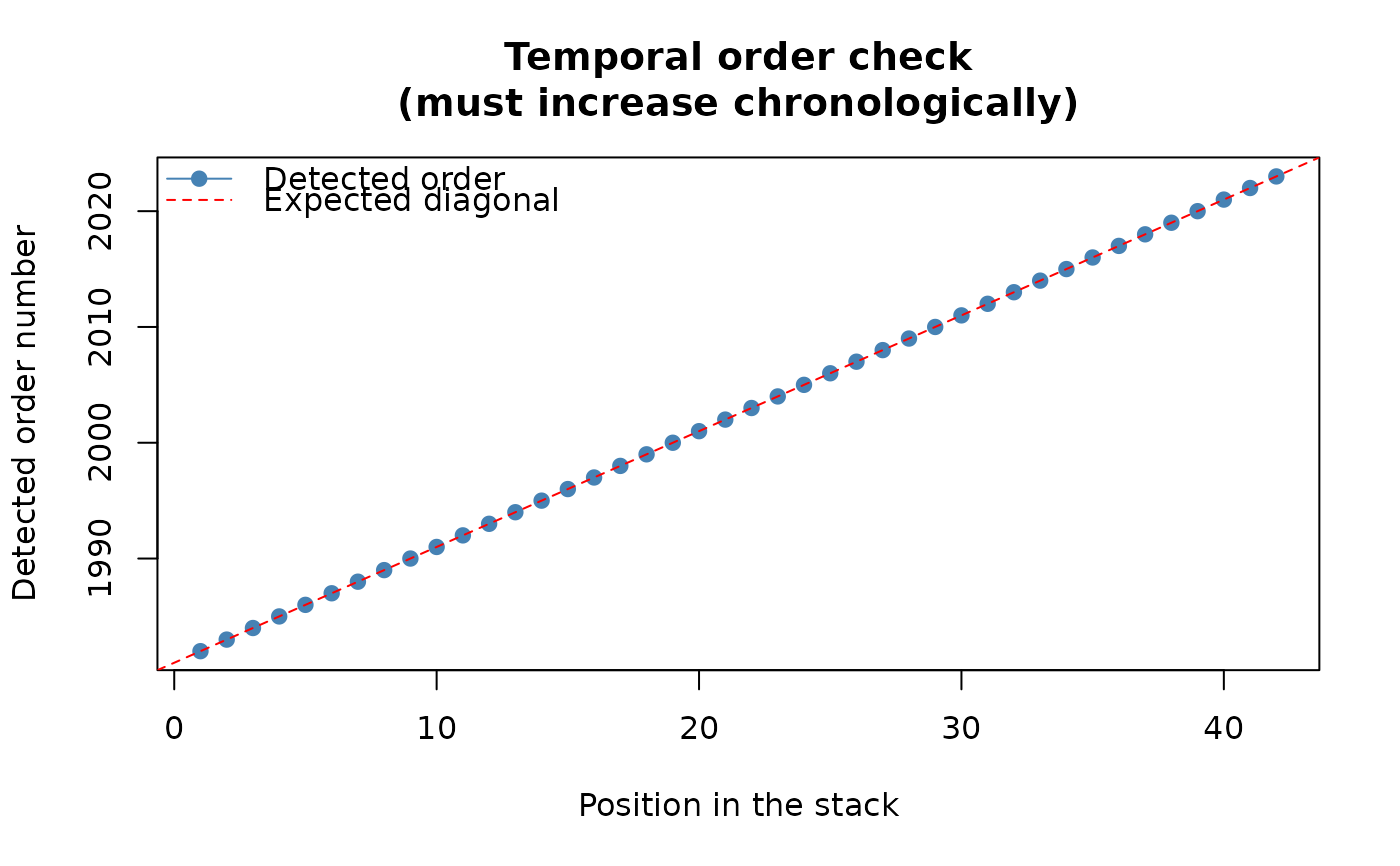 #> Stack built: 42 layers, 146 x 338 cells.
#> >> [read_ordered_stack()] elapsed: 0.13 s
trend <- trend_test(r, report = FALSE, verbose = FALSE)
fdr_result <- fdr_correction(trend$stats$p, report = FALSE, verbose = FALSE)
# Combines "is it significant" (from fdr_result) with "which way is
# it going" (from trend) into a single binarised trend map. Called
# internally by workflow_tst()/workflow_trends() to build the "TST/
# RTA direction map" panel automatically when report = TRUE (the
# default) -- there is no standalone public wrapper for this
# specific combination outside those workflows.
# direction <- direction_map(trend$stats, fdr_result, method = "BH")
# }
#> Stack built: 42 layers, 146 x 338 cells.
#> >> [read_ordered_stack()] elapsed: 0.13 s
trend <- trend_test(r, report = FALSE, verbose = FALSE)
fdr_result <- fdr_correction(trend$stats$p, report = FALSE, verbose = FALSE)
# Combines "is it significant" (from fdr_result) with "which way is
# it going" (from trend) into a single binarised trend map. Called
# internally by workflow_tst()/workflow_trends() to build the "TST/
# RTA direction map" panel automatically when report = TRUE (the
# default) -- there is no standalone public wrapper for this
# specific combination outside those workflows.
# direction <- direction_map(trend$stats, fdr_result, method = "BH")
# }