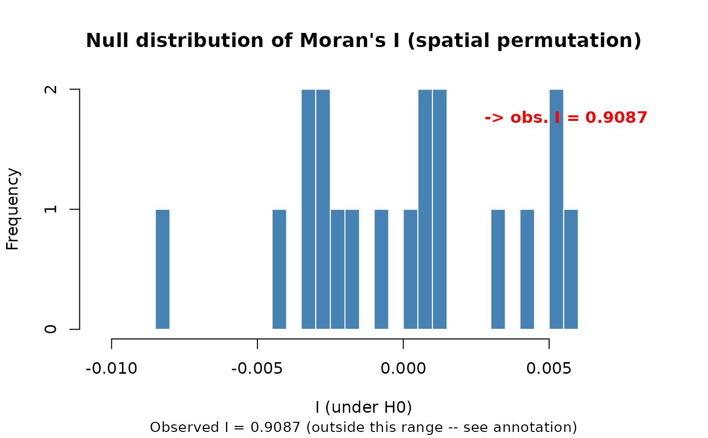
Null-distribution plot for a spatial_autocorrelation() result
Source:R/spatial_autocorrelation.R
spatial_autocorrelation_null_plot.RdFunction type: Reporting/derived function – summarises or
plots the output of
another function; it does not compute any new statistic. Not
exported – called internally by report = TRUE, and reachable from
outside the package via plot().
Arguments
- result
Output of
spatial_autocorrelation().- path
Character or
NULL. If supplied, write the table to this CSV path.
References
Moran, P.A.P. (1950) Notes on Continuous Stochastic Phenomena. Biometrika, 37(1-2), 17-23. doi:10.1093/biomet/37.1-2.17
Getis, A. and Ord, J.K. (1992) The Analysis of Spatial Association by Use of Distance Statistics. Geographical Analysis, 24(3), 189-206. doi:10.1111/j.1538-4632.1992.tb00261.x
See also
Other Spatial autocorrelation diagnostic functions:
classify_moran(),
spatial_autocorrelation(),
spatial_autocorrelation_summary()
Examples
r <- read_ordered_stack(example_data("vhp_ndvi"))[[1]]
#> Temporal order auto-detected with pattern '(19[0-9]{2}|20[0-9]{2})'.
#> Automatic mode: order detected from file names. For higher reliability -- especially if the series is not annual -- supplying 'files' explicitly (with 'time' or 'cycle_type') is recommended. See ?read_ordered_stack.
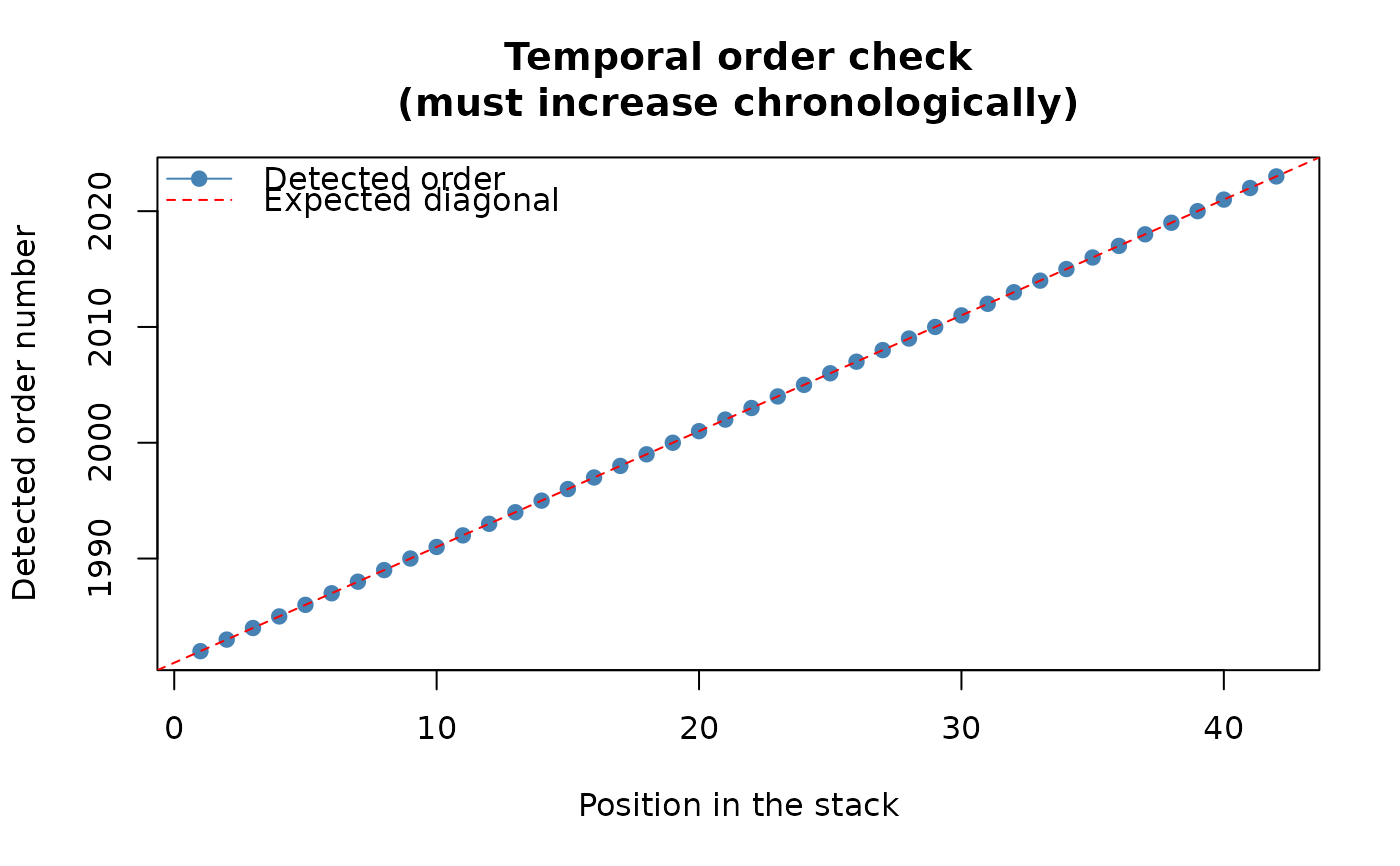
#> Temporal order verification (mandatory, cannot be skipped):
#> stack_position detected_number file
#> 1 1982 VHP_SMN_annual_ndvi_1982.tif
#> 2 1983 VHP_SMN_annual_ndvi_1983.tif
#> 3 1984 VHP_SMN_annual_ndvi_1984.tif
#> 4 1985 VHP_SMN_annual_ndvi_1985.tif
#> 5 1986 VHP_SMN_annual_ndvi_1986.tif
#> 6 1987 VHP_SMN_annual_ndvi_1987.tif
#> 7 1988 VHP_SMN_annual_ndvi_1988.tif
#> 8 1989 VHP_SMN_annual_ndvi_1989.tif
#> 9 1990 VHP_SMN_annual_ndvi_1990.tif
#> 10 1991 VHP_SMN_annual_ndvi_1991.tif
#> 11 1992 VHP_SMN_annual_ndvi_1992.tif
#> 12 1993 VHP_SMN_annual_ndvi_1993.tif
#> 13 1994 VHP_SMN_annual_ndvi_1994.tif
#> 14 1995 VHP_SMN_annual_ndvi_1995.tif
#> 15 1996 VHP_SMN_annual_ndvi_1996.tif
#> 16 1997 VHP_SMN_annual_ndvi_1997.tif
#> 17 1998 VHP_SMN_annual_ndvi_1998.tif
#> 18 1999 VHP_SMN_annual_ndvi_1999.tif
#> 19 2000 VHP_SMN_annual_ndvi_2000.tif
#> 20 2001 VHP_SMN_annual_ndvi_2001.tif
#> 21 2002 VHP_SMN_annual_ndvi_2002.tif
#> 22 2003 VHP_SMN_annual_ndvi_2003.tif
#> 23 2004 VHP_SMN_annual_ndvi_2004.tif
#> 24 2005 VHP_SMN_annual_ndvi_2005.tif
#> 25 2006 VHP_SMN_annual_ndvi_2006.tif
#> 26 2007 VHP_SMN_annual_ndvi_2007.tif
#> 27 2008 VHP_SMN_annual_ndvi_2008.tif
#> 28 2009 VHP_SMN_annual_ndvi_2009.tif
#> 29 2010 VHP_SMN_annual_ndvi_2010.tif
#> 30 2011 VHP_SMN_annual_ndvi_2011.tif
#> 31 2012 VHP_SMN_annual_ndvi_2012.tif
#> 32 2013 VHP_SMN_annual_ndvi_2013.tif
#> 33 2014 VHP_SMN_annual_ndvi_2014.tif
#> 34 2015 VHP_SMN_annual_ndvi_2015.tif
#> 35 2016 VHP_SMN_annual_ndvi_2016.tif
#> 36 2017 VHP_SMN_annual_ndvi_2017.tif
#> 37 2018 VHP_SMN_annual_ndvi_2018.tif
#> 38 2019 VHP_SMN_annual_ndvi_2019.tif
#> 39 2020 VHP_SMN_annual_ndvi_2020.tif
#> 40 2021 VHP_SMN_annual_ndvi_2021.tif
#> 41 2022 VHP_SMN_annual_ndvi_2022.tif
#> 42 2023 VHP_SMN_annual_ndvi_2023.tif
 #> Stack built: 42 layers, 146 x 338 cells.
#> >> [read_ordered_stack()] elapsed: 0.11 s
moran_result <- spatial_autocorrelation(r, nperm = 19, seed = 1,
verbose = FALSE, report = FALSE)
# The null distribution (I values from randomly shuffled data), with
# the observed I marked -- how unusual is it compared to pure chance?
# Called internally by plot() on a spatial_autocorrelation() result
# -- the public entry point is:
plot(moran_result)
#> Stack built: 42 layers, 146 x 338 cells.
#> >> [read_ordered_stack()] elapsed: 0.11 s
moran_result <- spatial_autocorrelation(r, nperm = 19, seed = 1,
verbose = FALSE, report = FALSE)
# The null distribution (I values from randomly shuffled data), with
# the observed I marked -- how unusual is it compared to pure chance?
# Called internally by plot() on a spatial_autocorrelation() result
# -- the public entry point is:
plot(moran_result)